A Gentle Introduction to the Python Binance API

Python-binance is an application programming interface that allows you to connect to the Binance servers via the Python programming language. It is important to note that the python-binance library is not affiliated with Binance.

This tutorial will show you how to extract and analyze real-time securities and crypto data from Binance using the python-binance API and Pandas library.

Prerequisites

To follow along, a reader needs to be familiar with:

• Python programming language.
• The Binance cryptocurrency exchange.
• Pandas and Matplotlib libraries.

The Python-Binance API

Binance is currently the largest cryptocurrency exchange in the world as far as daily trading volumes in concerned. It was founded in 2017 by Changpeng Zhao, and its headquarters is in the Cayman Islands. It allows you to easily buy, sell, trade, and swap cryptocurrency.

Python-binance is an application programming interface that allows you to connect to the Binance servers via the Python programming language. With the API, you can make orders, trade, withdraw and get real-time data from the Binance exchange. Feel free to read their documentation.

Setting up the Binance API

We first need to set up an API key by registering an account on Binance. This step involves heading to the Binance website and signing up if you don’t have an account with them yet. Registration is straightforward, as you would register for any web application. After successfully signing up and completing the verification process, hover over the profile button and select the API Management option as shown below:

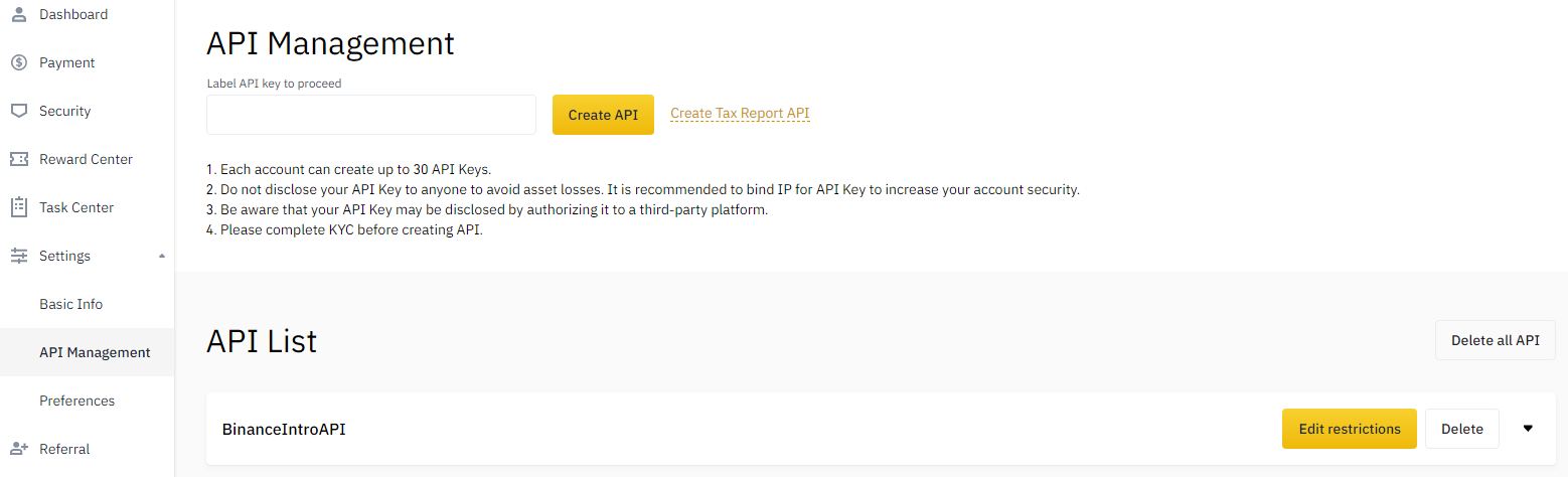
The API management is the option where you will be allowed to set up your API key. Once opened, you need to label the API you want to create, then click on the Create API button. For our case, we created one with the label, BinanceIntroAPI. After pressing the Create API button, you will be prompted to perform security verification quickly. Once done, your API key will be created successfully. You will get an API key and a secret key.

We need to make our account secure. You’ll see a button called Edit restrictions on the top right corner. Once inside, uncheck the Enable Spot & Margin Trading option and check the Restrict access to trusted IPs only (Recommended) option. Enter your IP address, then click save. If you don’t know your IP address, you can perform a quick search on Google for my ip address. This will take away the trading permissions and only limit access to a computer with your IP address.

Copy this API key and paste it on your notebook as shown below:

apikey = 'ENTERYOURAPIKEY'
apisecret = 'ENTERYOURSECRETKEY'

We’ve stored our API and secret keys in the apikey and apisecret variables.

Installing and importing dependencies

In this next step, we’ll go ahead and install and import the necessary dependencies.

!pip install python-binance pandas mplfinance

We’ve installed three dependencies:

• python-binance allows us to connect to the Binance API.
• pandas library will allow us to transform the crypto data.
• mplfinance will enable us to visualize financial data easily.

Let’s now import them into our notebook.

from binance import Client, ThreadedWebsocketManager, ThreadedDepthCacheManager
import pandas as pd

Performing authentication

Using the Client class we imported earlier, we import the two variables, apikey, and apisecret keys, to perform authentication. Then, we store this result in a variable called client.

client = Client(apikey, apisecret)

Pulling data from binance using Python-Binance

This step involves retrieving data from the API using the python-binance library.

Getting ticker data

tickers = client.get_all_tickers()
tickers

The function, get_all_tickers(), allows us to go ahead and grab all ticker values. There are a lot of other functions available for use to manage your account and place trades.

Output:

 {'price': '5.47400000', 'symbol': 'ANTUSDT'},
 {'price': '0.00687000', 'symbol': 'CRVBNB'},
 {'price': '0.00006287', 'symbol': 'CRVBTC'},
 {'price': '4.12300000', 'symbol': 'CRVBUSD'},
 {'price': '4.12100000', 'symbol': 'CRVUSDT'},
 {'price': '0.00442100', 'symbol': 'SANDBNB'},
 {'price': '0.00004385', 'symbol': 'SANDBTC'},
 {'price': '2.87380000', 'symbol': 'SANDUSDT'},
 {'price': '2.87510000', 'symbol': 'SANDBUSD'},
 {'price': '0.00144600', 'symbol': 'OCEANBNB'},
 ...

Performing EDA with Binance data

We’ll perform some exploratory data analysis on Binance data using the Pandas library.

ticker_dataframe = pd.DataFrame(tickers)
ticker_dataframe.head()

The output we get from running the code above is as follows:

  symbol  price
0   ETHBTC  0.07133100
1   LTCBTC  0.00417000
2   BNBBTC  0.00992500
3   NEOBTC  0.00074700
4   QTUMETH 0.00368000

As we’ve seen, the Pandas library makes it easy to work with data as it organizes it into data frames.

Getting depth data

depth = client.get_order_book(symbol='ETHUSDT')
depth

The get_order_book() function allows us to retrieve market depth data from Binance. You can change the crypto pair you want to retrieve data. For example, instead of the ETHUSDT pair, you could try a BTCUSDT or a BNBBTC pair.

Output:

['4667.44000000', '0.01470000'],
  ['4667.43000000', '1.36750000'],
  ['4667.42000000', '0.69830000'],
  ['4667.41000000', '0.08100000'],
  ['4667.40000000', '0.00990000'],
  ['4667.39000000', '0.02000000'],
  ['4667.38000000', '0.70130000']],
 'lastUpdateId': 12445843339}

Let’s visualize this data using Pandas.

depth_dataframe = pd.DataFrame(depth['asks'])
depth_dataframe.columns = ['Price', 'Volume']
depth_dataframe.head()

Output:

            Price   Volume
0   4671.90000000   7.19000000
1   4671.99000000   0.10000000
2   4672.00000000   0.30000000
3   4672.14000000   0.10700000
4   4672.15000000   0.10700000

Getting historical data

This next step involves getting some historical data and preprocessing them. This process is essential as the data isn’t appropriate for performing calculations. But, first, let’s take a look at the current data types:

depth_dataframe.dtypes

Price     object
Volume    object
dtype: object

As we’ve seen, the data is stored as objects. We’ll need to convert this data to numerical to perform calculations on them.

historical_data = client.get_historical_klines('BTCUSDT', Client.KLINE_INTERVAL_1DAY, '5 July 2020')

The get_historical_klines() function allows you to retrieve Spot and Futures data from Binance. It takes three parameters, the name of symbol pair, interval, and date. The function returns a limit of 1000 rows of data.

As for the interval time, there are many options you can play around with, i.e., KLINE_INTERVAL_1MINUTE, KLINE_INTERVAL_15MINUTE, KLINE_INTERVAL_1MONTH, KLINE_INTERVAL_1WEEK, etc.

If you want to build a trading bot, make sure to grab historical data from a date far back to build a model that works better.

If we take a look at this historical_data, this is what it contains:

historical_data

...
[1636675200000,
  '64774.25000000',
  '65450.70000000',
  '62278.00000000',
  '64122.23000000',
  '44490.10816000',
  1636761599999,
  '2844286547.50404090',
  1479149,
  '21028.45541000',
  '1344883879.13873450',
  '0'],
...

These values are stored inside a dictionary with the first 12 values for each trade representing:

1. Open Time
2. Open
3. High
4. Low
5. Close
6. Volume
7. Close Time
8. Quote Asset Volume
9. Number of Trades
10. Taker buy base asset volume
11. Taker buy quote asset volume
12. Ignore

Rather than leaving the data as is, we can put this data into a Pandas data frame.

hist_df = pd.DataFrame(historical_data)

When we run the hist_df.tail(), this is what it contains:

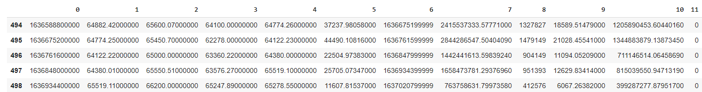
Rather than having numbers as our column names, we could rename these columns using Pandas column attribute.

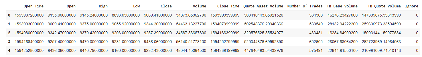
hist_df.columns = ['Open Time', 'Open', 'High', 'Low', 'Close', 'Volume', 'Close Time', 'Quote Asset Volume', 
                    'Number of Trades', 'TB Base Volume', 'TB Quote Volume', 'Ignore']

To visualize it, we write the following code:

hist_df.head()

Output:

If we type hist_df.dtypes, we’ll notice that more than half of the columns are stored as objects (string). Since we are working with financial data and want to do computations, we need to convert this into numerical values.

Preprocessing historical data

hist_df.dtypes

Output:

Open Time              int64
Open                  object
High                  object
Low                   object
Close                 object
Volume                object
Close Time             int64
Quote Asset Volume    object
Number of Trades       int64
TB Base Volume        object
TB Quote Volume       object
Ignore                object
dtype: object

We begin by converting the Open Time and Close Time to date-time values. We’ll use the to_datetime() function from pandas to do this. As dates are returned from Binance as timestamps, we first divide by 1000 and then set the units to seconds to convert correctly.

hist_df['Open Time'] = pd.to_datetime(hist_df['Open Time']/1000, unit='s')
hist_df['Close Time'] = pd.to_datetime(hist_df['Close Time']/1000, unit='s')

Now, let’s go ahead and convert our objects into numerical values using the to_numeric function.

numeric_columns = ['Open', 'High', 'Low', 'Close', 'Volume', 'Quote Asset Volume', 'TB Base Volume', 'TB Quote Volume']
hist_df[numeric_columns] = hist_df[numeric_columns].apply(pd.to_numeric, axis=1)

We have created a variable called numeric_columns. This variable stores the list of the data we want to convert into numeric. We then use the apply() method to perform this converstion.

We can take a look at the results by issuing the command, hist_df.head():

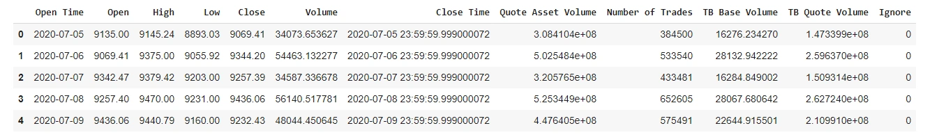
After transforming the data types, we can view the new data types using the command, hist_df.dtypes:

Open Time             datetime64[ns]
Open                         float64
High                         float64
Low                          float64
Close                        float64
Volume                       float64
Close Time            datetime64[ns]
Quote Asset Volume           float64
Number of Trades               int64
TB Base Volume               float64
TB Quote Volume              float64
Ignore                        object
dtype: object

We’ve successfully preprocessed the historical data. Additionally, you can do other types of analysis on the data. Play around with hist_df.describe() and hist_df.info to see what you can find.

Visualization using matplotlib finance library

This step will explore and visualize data using mplfinance. It is a financial market data visualization tool built on top of matplotlib.

We begin by importing the library into our notebook.

import mplfinance as mpf

We will visualize the Close Time data and limit the data to only the last 100 rows. In the plot, we’ve also included the candlestick type of plotting, volume data, the title for our plot, and finally, the 10, 20, and 30 moving day averages.

mpf.plot(hist_df.set_index('Close Time').tail(100), 
        type='candle', style='charles', 
        volume=True, 
        title='BTCUSDT Last 100 Days', 
        mav=(10,20,30))

Output:

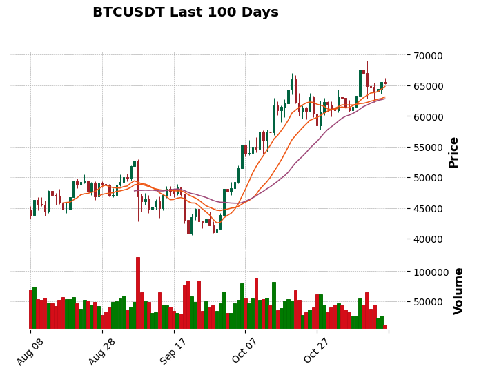
As we’ve seen, the matplotlib finance library allows us to visualize data easily.

Please find the code for this tutorial here.

Summary

In a nutshell, this tutorial has shown you what’s possible with the python-binance API. In addition, we’ve shown you how you can perform an exploratory data analysis on Binance data. In our follow-up tutorial, we’ll build upon this tutorial and show you how to apply machine learning and data science to trading and finance.

Further reading

• Mplfinance