Multivariate Time Series using Auto ARIMA

A time series is a collection of continuous data points recorded over time. It has equal intervals such as hourly, daily, weekly, minutes, monthly, and yearly.

Examples of time series data include annual budgets, company sales, weather records, air traffic, Covid-19 caseloads, forex exchange rates, and stock prices.

A time series model analyzes time series values and identifies hidden patterns. Eventually, the model predicts future time series values based on previously observed/historical values.

In this tutorial, we will build on a multivariate time series model. The model will learn using multiple variables. We create the model using Auto ARIMA.

Prerequisites

For a reader to understand the time series concepts explained in this tutorial, they should understand:

• Introduction to time series
• Time Series decomposition
• Building a simple time series application
• How to run the Python code in Google Colab

Getting started with Auto ARIMA

Auto ARIMA is a time series library that automates the process of building a model using ARIMA. Auto ARIMA applies the concepts of ARIMA in modeling and forecasting.

Auto ARIMA automatically finds the best parameters of an ARIMA model. To follow along with this tutorial, you have to understand the concepts of the ARIMA model.

Understanding the ARIMA model

Auto-Regressive Integrated Moving Average (ARIMA) is a time series model that identifies hidden patterns in time series values and makes predictions. For example, an ARIMA model can predict future stock prices after analyzing previous stock prices.

Also, an ARIMA model assumes that the time series data is stationary. Before implementing the ARIMA model, we will remove the non-stationarity components in the time series.

How to remove non-stationarity components in a time series

A non-stationary time series is a series whose properties change over time. A non-stationary time series has trends and seasonality components. Removing the non-stationarity in a time series will make it stationary and apply the ARIMA model.

The properties of time series that should remain constant are variance and mean. Allowing these properties to remain constant will remove the trend and seasonal components. We remove non-stationarity in a time series through differencing.

The differencing technique subtracts the present time series values from the past time series values. We may have to repeat the process of differencing multiple times until we output a stationary time series.

An ARIMA model has three initials: AR, I, and MA. These initials represent the three sub-models that form a single uniform model. The function of the initials is as follows:

Explaining ARIMA initials

AR – Auto Regression. I – Integrated. MA – Moving average.

They have the following functionalities:

• Auto Regression sub-model – This sub-model uses past values to make future predictions.
• Integrated sub-model – This sub-model performs differencing to remove any non-stationarity in the time series.
• Moving Average sub-model. – It uses past errors to make a prediction.

These sub-models are parameters of the overall ARIMA model. We initialize the parameters using unique notations as follows:

• p: It is the order of the Auto Regression (AR) sub-model. It refers to the number of past values that the model uses to make predictions.
• d: It is the number of differencing done to remove non-stationary components.
• q: It is the order of the Moving Average (MA) sub-model. It refers to the number of past errors that an ARIMA Model can have when making predictions.

Why do we use Auto ARIMA?

Before we build an ARIMA model, we pass the p,d, and q values. We use statistical plots and techniques to find the optimal values of these parameters.

We also use statistical plots such as Partial Autocorrelation Function plots and AutoCorrelation Function plot.

The process of using statistical plots is usually hectic and time-consuming. Many people have difficulties interpreting these plots to find the optimal parameter values. Wrong interpretation leads to people not getting the best/optimal p,d, and q values. It affects the ARIMA model’s overall performance.

Auto ARIMA automatically generates the optimal parameter values (p,d, and q). The generated values are the best, and the model will give accurate forecast results.

Auto ARIMA simplifies the process of building a time series model using the ARIMA model. Now we know how an ARIMA works and how Auto ARIMA applies its concepts. We will start exploring the time series dataset.

Energy consumption dataset

We will use the energy consumption dataset to build the Auto ARIMA model. The dataset shows the energy demand from 2012 to 2017 recorded in an hourly interval.

Download the time series dataset using this link. After downloading the time series dataset, we will load it using the Pandas library.

import pandas as pd

To load the energy consumption dataset, run this code:

df = pd.read_csv('energy_consumption.csv')

To visualize the dataset, use this code:

df

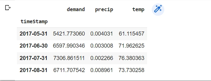
Energy consumption dataset output:

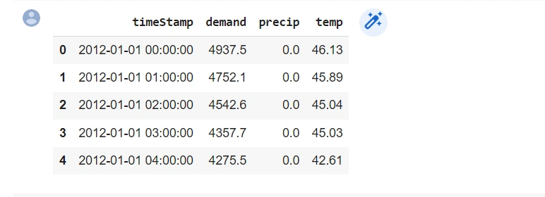
From this output, we have the timeStamp, demand, precip, and temp columns. The columns are the variables that will build the time series model.

The time series is multivariate since it has three-time dependent variables (demand, precip, and temp). They have the following functions:

• The timestamp column shows the time of recording.
• The demand column shows the hourly energy consumption.
• The precip and temp columns correlate with the demand column.

Converting the timestamp column

We need to convert the timestamp column to the DateTime format. It will enable us to perform time-series analysis and operations on this column. We will use the pd.to_datetime function.

df['timeStamp']=pd.to_datetime(df['timeStamp'])

Plotting the demand column

Since we are forecasting the demand, we plot this column to visualize the data points. It will enable us to check for trends or seasonality in the time series. We will use the Plotly Express Python module to plot the line chart.

We import the Plotly Express Python module as follows:

import plotly.express as px

To plot the demand column, use the following code:

fig = px.line(df, x='timeStamp', y='demand', title='Energy Consumption')

fig.update_xaxes(
    rangeslider_visible=True,
    rangeselector=dict(
        buttons=list([
            dict(step="all")
        ])
    )
)
fig.show()

It plots the following line chart:

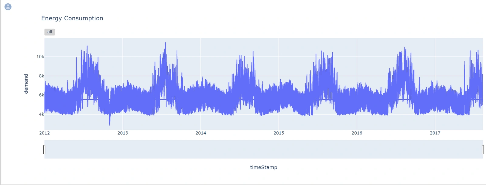
From the output above, the dataset has seasonality (repetitive cycles). Since the dataset has seasonality, we can say it is non-stationary. But still, we need to perform a statistical check using the Augmented Dickey-Fuller (ADF) test to assess stationarity in our dataset. The test is more accurate.

If we find the dataset is non-stationary after the ADF test, we will have to perform differencing to make it stationary. Auto ARIMA performs differencing automatically. The next step is to set the timeStamp as the index column.

el_df=df.set_index('timeStamp')

We set the timeStamp as the index column for better interaction with the data frame. The Auto ARIMA model also expects the timeStamp to be the index column.

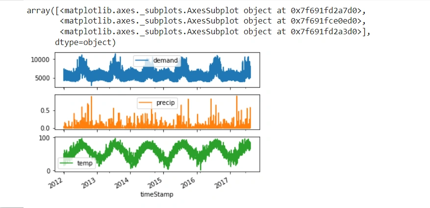
Plotting subplots

The subplots will show the time-dependent variables in the dataset. We will visualize the demand, precip, and temp columns.

el_df.plot(subplots=True)

It produces the following subplots:

Checking for missing or null values

We need to check for missing values in the dataset. Missing values affects the model and leads to inaccurate forecast results.

print ("\nMissing values :  ", df.isnull().any())

Output:

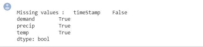
From the output, all the columns have missing values. We will handle the missing values using data imputation. It ensures we have a complete-time series dataset.

Imputing missing values

We will first impute the missing values in the demand column. We will use the fillna method.

Imputing ‘demand’ column

df['demand']=df['demand'].fillna(method='ffill')

Imputing ’temp’ column

df['temp']=df['temp'].fillna(method='ffill')

Imputing ‘precip’ column

df['temp']=df['precip'].fillna(method='ffill')

To learn more on how to handle missing values in time series using data imputation, go through this article

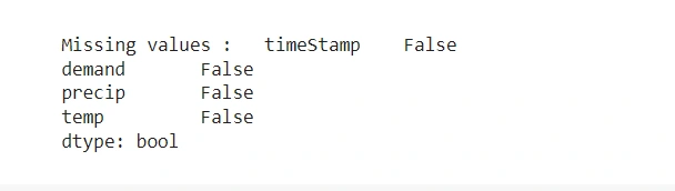
We check again for missing values to know if we have handled the issue successfully.

print ("\nMissing values :  ", df.isnull().any())

Dataset resampling

The time series has many data points that may be difficult to analyze and visualize. We need to resample the time by compressing and aggregating it to monthly intervals. We will have fewer data points that are easier to analyze.

The resample() method will aggregate all the data points in the time series and change them to monthly intervals.

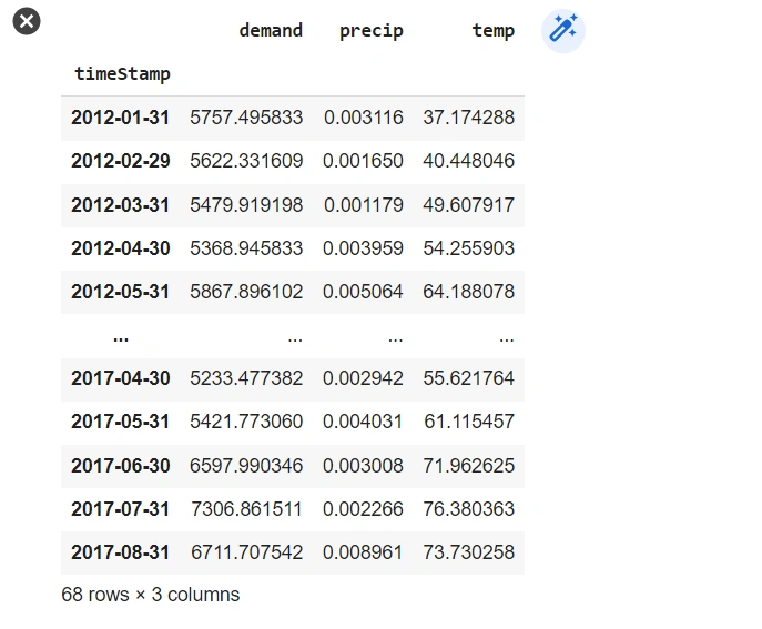
el_df.resample('M').mean()

Dataset resampling output:

Let’s plot new subplots of the resampled dataset.

Plotting new subplots

We plot the new subplot as follows:

el_df.resample('M').mean().plot(subplots=True)

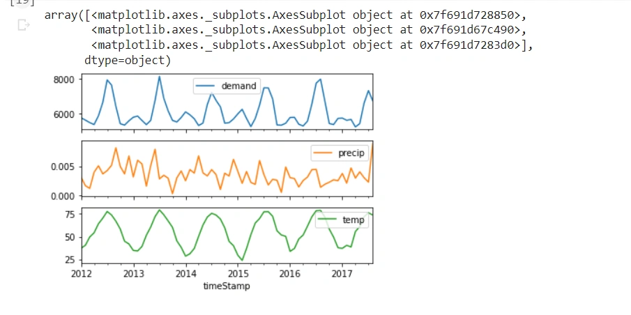
From these new subplots, we have resampled the dataset. It will be easier to model these fewer data points. We will save the resampled dataset in a new variable.

Saving the resampled dataset

We save the resampled dataset as follows:

final_df=el_df.resample('M').mean()

We will use this dataset to train the time series model. We can now start implementing the Auto ARIMA model.

Implementing the Auto ARIMA model

We implement the Auto ARIMA model using the pmdarima time-series library. This library provides the auto_arima() function that automatically generates the optimal parameter values.

To install pmdarima, use this command:

!pip install pmdarima

After the installation, we import it as follows:

import pmdarima as pm

The next step is to initialize the auto_arima() function.

Initialize the auto arima function

We initialize the auto_arima() function as follows:

model = pm.auto_arima(final_df['demand'], 
                        m=12, seasonal=True,
                      start_p=0, start_q=0, max_order=4, test='adf',error_action='ignore',  
                           suppress_warnings=True,
                      stepwise=True, trace=True)

In the auto_arima() function we pass the final_df which is our resampled dataset. We select the demand column since this is what the model wants to predict.

The function can either use the Grid Search technique, or Random Search technique to find the optimal parameter values. It tries multiple combinations of p,d, and q and then selects the optimal ones.

The auto_arima() function also has the following parameters:

• m=12 – It represents the number of months in a year.
• start_p=0 – It represents the minimum p value that the function can select during the random search.
• start_q=0 – It represents the minimum q value that the function can select during the random search.
• max_order=4 – It represents the maximum p, d, and q values that the model can select during the random search.
• test='adf' – It is an Augmented Dickey-Fuller (ADF) test to check for stationarity in our dataset. If the dataset is non-stationary after the ADF test, the auto_arima() function will automatically generate the d value for differencing. If the dataset is stationary, it sets d=0 (no need for differencing).
• suppress_warnings=True – It ignores the warnings during the parameter searching.
• stepwise=True – It will run the Random Search to find the optimal parameters. Grid Search is more exhaustive since it tries all the parameter combinations, but it is slow. We opt to use Random Search since it is faster.

When you run this code, the function will randomly search the parameters and produce the following output:

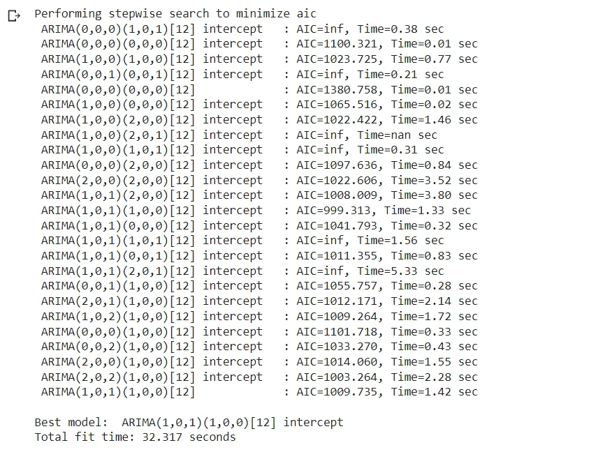
From the output above, the best model is ARIMA(1,0,1) (p=1, d=0, and q=1). The function automatically sets d=0 because the ADF test found the dataset is stationary.

We had previously observed the time series dataset plots to have seasonality. Therefore, we thought the time series was non-stationary, hence a need for differencing.

But using the ADF test, which is a statistical test, found the seasonality is insignificant. ADF test is more accurate than observing/visualizing the plots. That is why the function sets d=0, and there is no need for differencing.

After initializing the auto_arima() function, the next step is to split the time series dataset.

Splitting the time series dataset

We split the time series dataset into a training data frame and a test data frame as follows:

train=final_df[(final_df.index.get_level_values(0) >= '2012-01-31') & (final_df.index.get_level_values(0) <= '2017-04-30')]

The code selects the data points from 2012-01-31 to 2017-04-30 for model training. We get the data points for model testing using the following code:

test=final_df[(final_df.index.get_level_values(0) > '2017-04-30')]

The data points from 2017-04-30 are for model testing. To display the test data points, use this code:

test

From the output, the test data frame has four data points.

Let’s fit the Auto ARIMA model to the train data frame.

Fitting the Auto ARIMA model

Fitting the Auto ARIMA model to the train data frame will enable the model to learn from the time-series dataset. The final model will make future predictions.

model.fit(train['demand'])

After training, it produces the following output:

We train the model using the train data frame. It also uses the optimal p,d, and q parameter values during training. Let’s use the model to make predictions.

Using the Auto ARIMA model to make predictions

The Auto ARIMA model will predict using the test data frame. It will also forecast/predict the unseen future time series values.

Predicting the test data frame

We predict the test data frame as follows:

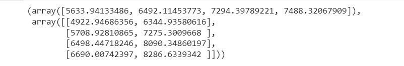
forecast=model.predict(n_periods=4, return_conf_int=True)

• n_periods=4: It represents the number of the data points in the test data frame that the model will predict. To see the predicted values, use this code:

forecast

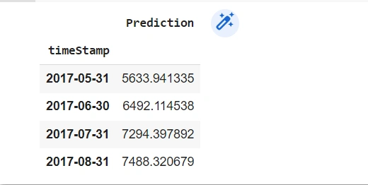
We need to convert the predicted values to a Pandas data frame. It will be easier to plot the Pandas data frame using Matplotlib.

forecast_df = pd.DataFrame(forecast[0],index = test.index,columns=['Prediction'])

To see the Pandas data frame, run this code:

forecast_df

It produces this output:

The next step is to plot the Pandas data frame using Matplotlib.

Plotting the Pandas data frame

We import Matplotlib as follows:

import matplotlib.pyplot as plt

We plot the line chart as follows:

pd.concat([final_df['demand'],forecast_df],axis=1).plot()

It produces the following line chart:

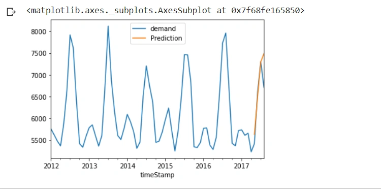
From the line chart above:

• The blue line is the actual energy demand.
• The orange line is the predicted energy demand.

The Auto ARIMA model has performed well and has made accurate predictions. The blue and orange lines are close to each other.

We can now use this model to predict unseen future values.

Predict the unseen future time series values

To predict/forecast the unseen future values, use this code:

forecast1=model.predict(n_periods=8, return_conf_int=True)
forecast_range=pd.date_range(start='2017-05-31', periods=8,freq='M')

• n_periods=8 It represents the number of data points the model will predict in the future. The future dates are from 2017-05-31. We also need to convert the predicted values to a Pandas data frame.

forecast1_df = pd.DataFrame(forecast1[0],index =forecast_range,columns=['Prediction'])

Finally, we plot the future predicted values using Matplotlib

Plotting the future predicted values

To plot the future predicted values, use the following code:

pd.concat([final_df['demand'],forecast1_df],axis=1).plot()

It produces the following line chart:

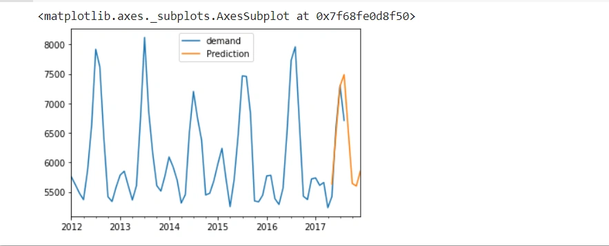
From the line chart above:

• The blue line represents the actual energy demand.
• The orange line represents the predicted energy demand.

The orange line also shows the unseen future predictions. The Auto ARIMA model has performed well since the orange line maintains the general pattern.

Conclusion

In this tutorial, We have learned how to build a multivariate time series model with Auto ARIMA. We explored how the Auto ARIMA model works and how it automatically finds the best parameters of an ARIMA model.

Finally, we implemented the Auto ARIMA model. We used the Auto ARIMA model to find the p, d, and q values.

We used the trained Auto ARIMA model to predict the energy demand on the test data frame and the unseen future time series values. The final model made accurate predictions observed in the plotted line chart.

You can get the complete Python implementation of this tutorial in Google Colab here

Further reading

• Auto ARIMA documentation
• Pmdarima documentation
• What is auto ARIMA?
• ARIMA Model time series forecasting
• ARIMA model definition
• Hyperparameter Tuning
• Random Search technique
• Grid Search technique
• ARIMA model guide
• ARIMA models