DBSCAN Algorithm Clustering in Python

DBSCAN is a popular density-based data clustering algorithm. To cluster data points, this algorithm separates the high-density regions of the data from the low-density areas. Unlike the K-Means algorithm, the best thing with this algorithm is that we don’t need to provide the number of clusters required prior.

DBSCAN algorithm in Python

DBSCAN algorithm group points based on distance measurement, usually the Euclidean distance and the minimum number of points. An essential property of this algorithm is that it helps us track down the outliers as the points in low-density regions; hence it is not sensitive to outliers as is the case of K-Means clustering.

Prerequisites

To follow along the reader will need the following:

1. Python installed on your system or access to the Google Colab.
2. A Dataset available in the form of a CSV file.

Introduction

DBSCAN algorithm works with two parameters.

These parameters are:

1. Epsilon (Eps): This is the least distance required for two points to be termed as a neighbor. This distance is known as Epsilon (Eps). Thus we consider Eps as a threshold for considering two points as neighbors, i.e., if the distance between two points is utmost Eps, then we consider the two points to be neighbors.
2. MinPoints: This refers to the minimum number of points needed to construct a cluster. We consider MinPoints as a threshold for considering a cluster as a cluster. A cluster is only recognized if the number of points is greater than or equal to the MinPts.

We classify data points into three categories based on the two parameters above. So let us look at these categories.

Types of data points in a DBSCAN clustering

After the DBSCAN clustering is complete, we end up with three types of data points as follows:

1. Core: This is a point from which the two parameters above are fully defined, i.e., a point with at least Minpoints within the Eps distance from itself.
2. Border: This is any data point that is not a core point, but it has at least one Core point within Eps distance from itself.
3. Noise: This is a point with less than Minpoints within distance Eps from itself. Thus, it’s not a Core or a Border.

Let’s now look at the algorithmic steps of DBSCAN clustering.

DBSCAN algorithm

The following are the DBSCAN clustering algorithmic steps:

• Step 1: Initially, the algorithms start by selecting a point (x) randomly from the data set and finding all the neighbor points within Eps from it. If the number of Eps-neighbours is greater than or equal to MinPoints, we consider x a core point. Then, with its Eps-neighbours, x forms the first cluster.

After creating the first cluster, we examine all its member points and find their respective Eps -neighbors. If a member has at least MinPoints Eps-neighbours, we expand the initial cluster by adding those Eps-neighbours to the cluster. This continues until there are no more points to add to this cluster.

• Step 2: For any other core point not assigned to cluster, create a new cluster.
• Step 3: To the core point cluster, find and assign all points that are recursively connected to it.
• Step 4: Iterate through all unattended points in the dataset and assign them to the nearest cluster at Eps distance from themselves. If a point does not fit any available clusters, locate it as a noise point.

Python implementation of DBSCAN

As usual to any implementation, we get started with fetching the dataset and preparing it ready for our model implementation. However, first, let us download this data here.

Data Preprocessing

Importing the required libraries

Let us begin by importing the required libraries for implementation on the algorithm.

import numpy as np
import matplotlib.pyplot as plt
import pandas as pd
data = pd.read_csv("/content/drive/MyDrive/Mall_Customers.csv") # importing the dataset

Exploratory data analysis

This is the process of investigating the available data and determining inconsistencies in patterns and other anomalies with the help of graphical representations and statistical summaries.

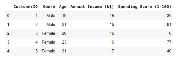
• Checking the head of the data.

data.head()

• Output

• Checking the shape of the dataset.

print("Dataset shape:", data.shape)

Output

Dataset shape: (200, 5)

Next, we check if the dataset has any missing values.

# checking for NULL data in the dataset
data.isnull().any().any()

Output

False

The above output means there are no missing values in our dataset. Since our data is ready to use, let us extract the Annual Income and the Spending Score columns and apply our DBSCAN model to them.

# extracting the above mentioned columns
x = data.loc[:, ['Annual Income (k$)',
                 'Spending Score (1-100)']].values

• Let us check the shape of x.

print(x.shape)

Output

(200, 2)

Before we apply the DBSCAN model, first, we need to obtain its two parameters.

1. MinPoints: We can obtain the minimum number of Points to be used to recognize a cluster, as follows:

• If the dataset has two dimensions, use the min sample per cluster as 4.
• If the data has more than two dimensions, the min sample per cluster should be: Min_sample(MinPoints) = 2 * Data dimension

Since our data is two-dimensional, we shall use the default value of 4 as our MinPoint parameter.

2. Epsilon (Eps): To calculate the value of Eps, we shall calculate the distance between each data point to its closest neighbor using the Nearest Neighbours. After that, we sort them and finally plot them. From the plot, we identify the maximum value at the curvature of the graph. This value is our Eps.

Compute data proximity from each other using Nearest Neighbours

from sklearn.neighbors import NearestNeighbors # importing the library
neighb = NearestNeighbors(n_neighbors=2) # creating an object of the NearestNeighbors class
nbrs=neighb.fit(x) # fitting the data to the object
distances,indices=nbrs.kneighbors(x) # finding the nearest neighbours

Sorting and plot the distances between the data points

# Sort and plot the distances results
distances = np.sort(distances, axis = 0) # sorting the distances
distances = distances[:, 1] # taking the second column of the sorted distances
plt.rcParams['figure.figsize'] = (5,3) # setting the figure size
plt.plot(distances) # plotting the distances
plt.show() # showing the plot

Output

Executing the code above, we obtain the following plot:

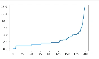
From the above plot, we note the maximum curvature of the curve is about eight, and thus we picked our Eps as 8.

We now have our two parameters as:

• MinPoints = 4
• Eps = 8

Now that we have the parameters let us implement the DBSCAN model.

Implementing the DBSCAN model

from sklearn.cluster import DBSCAN
# cluster the data into five clusters
dbscan = DBSCAN(eps = 8, min_samples = 4).fit(x) # fitting the model
labels = dbscan.labels_ # getting the labels

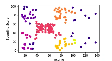
# Plot the clusters
plt.scatter(x[:, 0], x[:,1], c = labels, cmap= "plasma") # plotting the clusters
plt.xlabel("Income") # X-axis label
plt.ylabel("Spending Score") # Y-axis label
plt.show() # showing the plot

Clusters plot

Conclusion

In this article, we have covered the DBSCAN algorithm. First, we looked at its key parameters and how this algorithm clusters the data points. We also learned about three data points associated with the DBSCAN algorithm. Later we looked at how we implement this algorithm.

Happy coding.