Entropy and Information Gain to Build Decision Trees in Machine Learning

A decision tree is a supervised learning algorithm used for both classification and regression problems. Simply put, it takes the form of a tree with branches representing the potential answers to a given question. There are metrics used to train decision trees. One of them is information gain. In this article, we will learn how information gain is computed, and how it is used to train decision trees.

Prerequisites

If you are unfamiliar with decision trees, I recommend you read this article first for an introduction.

To follow along with the code, you’ll require:

• A code editor such as VS Code which is the code editor I used for this tutorial. The language we shall program in is Python.

• We shall use the scikit-learn library.

• Matplotlib comes in handy for the visualization of our tree.

• We use the iris dataset

Entropy

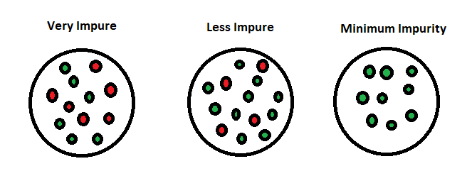
Entropy is an information theory metric that measures the impurity or uncertainty in a group of observations. It determines how a decision tree chooses to split data. The image below gives a better description of the purity of a set.

Source

Consider a dataset with N classes. The entropy may be calculated using the formula below:

$$E = - \sum\limits_{i=1}^{N} p_i log_2 p_i$$

$p_i$ is the probability of randomly selecting an example in class $i$. Let’s have an example to better our understanding of entropy and its calculation. Let’s have a dataset made up of three colors; red, purple, and yellow. If we have one red, three purple, and four yellow observations in our set, our equation becomes:

$$E = - ( p_r log_2 p_r + p_p log_2 p_p + p_y log_2 p_y )$$

Where $p_r$, $p_p$ and $p_y$ are the probabilities of choosing a red, purple and yellow example respectively. We have $p_r = \frac{1}{8}$ because only $\frac{1}{8}$ of the dataset represents red. $\frac{3}{8}$ of the dataset is purple hence $p_p = \frac{3}{8}$. Finally, $p_y = \frac{4}{8}$ since half the dataset is yellow. As such, we can represent $p_y$ as $p_y = \frac{1}{2}$. Our equation now becomes:

$$E = - ( \frac{1}{8} log_2 (\frac{1}{8}) + \frac{3}{8} log_2 (\frac{3}{8}) + \frac{4}{8} log_2 (\frac{4}{8}) )$$

Our entropy would be: $1.41$

You might wonder, what happens when all observations belong to the same class? In such a case, the entropy will always be zero.

$$E = - (1 log_2 1)$$

$$= 0$$

Such a dataset has no impurity. This implies that such a dataset would not be useful for learning. However, if we have a dataset with say, two classes, half made up of yellow and the other half being purple, the entropy will be one.

$$E = - ((0.5 log_2 0.5) + (0.5 log_2 0.5))$$

$$= 1$$

This kind of dataset is good for learning.

Information Gain

We can define information gain as a measure of how much information a feature provides about a class. Information gain helps to determine the order of attributes in the nodes of a decision tree.

The main node is referred to as the parent node, whereas sub-nodes are known as child nodes. We can use information gain to determine how good the splitting of nodes in a decision tree.

It can help us determine the quality of splitting, as we shall soon see. The calculation of information gain should help us understand this concept better.

$$Gain = E_{parent} - E_{children}$$

The term Gain represents information gain. $E_{parent}$ is the entropy of the parent node and E_{children} is the average entropy of the child nodes. Let’s use an example to visualize information gain and its calculation.

Suppose we have a dataset with two classes. This dataset has 5 purple and 5 yellow examples. The initial value of entropy will be given by the equation below. Since the dataset is balanced, we expect the answer to be $1$.

$$E_{initial} = - ((0.5 log_2 0.5) + (0.5 log_2 0.5))$$

$$= 1$$

Say we split the dataset into two branches. One branch ends up having four values while the other has six. The left branch has four purples while the right one has five yellows and one purple.

We mentioned that when all the observations belong to the same class, the entropy is zero since the dataset is pure. As such, the entropy of the left branch $E_{left} = 0$. On the other hand, the right branch has five yellows and one purple. Thus:

$$E_{right} = - ( \frac{5}{6} log_2 (\frac{5}{6}) + \frac{1}{6} log_2 (\frac{1}{6}) )$$

A perfect split would have five examples on each branch. This is clearly not a perfect split, but we can determine how good the split is. We know the entropy of each of the two branches. We weight the entropy of each branch by the number of elements each contains.

This helps us calculate the quality of the split. The one on the left has 4, while the other has 6 out of a total of 10. Therefore, the weighting goes as shown below:

$$E_{split} = 0.6 *0.65 + 0.4 *0$$

$$= 0.39$$

The entropy before the split, which we referred to as initial entropy $E_{initial} = 1$. After splitting, the current value is $0.39$. We can now get our information gain, which is the entropy we “lost” after splitting.

$$Gain = 1 – 0.39$$

$$= 0.61$$

The more the entropy removed, the greater the information gain. The higher the information gain, the better the split.

Using Information Gain to Build Decision Trees

Since we now understand entropy and information gain, building decision trees becomes a simple process. Let’s list them:

1. An attribute with the highest information gain from a set should be selected as the parent (root) node. From the image below, it is attribute A.

Source

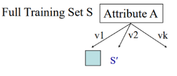
2. Build child nodes for every value of attribute A.

3. Repeat iteratively until you finish constructing the whole tree.

Decision tree example

Our goal is to visualize a decision tree through a simple Python example. Let’s begin!

For trees of greater complexity, you should expect to come across more parameters. However, since we are building as simple a decision tree as possible, these two parameters are the ones we use.

max_depth. Each decision tree has a maximum number of levels permitted. max_depth represents this number.

min_samples_leaf. The minimum sample count storable in a leaf node.

1. Import the required libraries

from sklearn.datasets import load_iris
from sklearn import tree
from matplotlib import pyplot as plt

2. Load the Iris dataset The Iris dataset is a very versatile dataset. It has three classes of irises, namely Setosa, Versicolour, and Virginica. Each class has fifty samples. The rows of this dataset are the samples. As for the columns, we have Sepal Length, Sepal Width, Petal Length, and Petal Width. We shall come across these features in our code.

from sklearn.datasets import load_iris
iris = load_iris()
X = iris.data
y = iris.target

3. Build and fit decision tree For this specific example, I used the following pair of lines.

clf = tree.DecisionTreeClassifier(criterion='entropy', max_depth=4,min_samples_leaf=4)
clf.fit(X,y)

Recall that we defined max_depth and min_samples_leaf earlier on. I encourage you to tinker with the values of each parameter and see how it affects the final plot.

4. Plot the decision tree.

fig, ax = plt.subplots(figsize=(6, 6))
tree.plot_tree(clf,ax=ax,feature_names=['sepal length','sepal width','petal length','petal width'])
plt.show()

Something worth noting here is that the value of figsize changes the size of the plotted outcome. Once more, I encourage you to tinker with this to your liking.

All the code

You may also find and experiment with all the code here.

from sklearn.datasets import load_iris
from sklearn import tree
from matplotlib import pyplot as plt
iris = load_iris()

X = iris.data
y = iris.target

#build decision tree
clf = tree.DecisionTreeClassifier(criterion='entropy', max_depth=4,min_samples_leaf=4)
#max_depth represents max level allowed in each tree, min_samples_leaf minumum samples storable in leaf node

#fit the tree to iris dataset
clf.fit(X,y)

#plot decision tree
fig, ax = plt.subplots(figsize=(6, 6)) #figsize value changes the size of plot
tree.plot_tree(clf,ax=ax,feature_names=['sepal length','sepal width','petal length','petal width'])
plt.show()

Results

We finally have our decision tree!

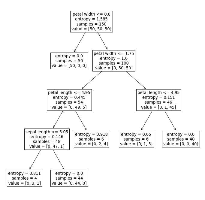
Remember to play around with the values of max_depth and min_samples_leaf to see how they change the resulting tree.

Wrapping up

Decision trees are one of the simplest machine learning algorithms to not only understand but also implement. We have learned how decision trees split their nodes and how they determine the quality of their splits.

We have also mentioned the basic steps to build a decision tree. Furthermore, we have shown this through a few lines of code.

I hope this article has given a simple primer on decision trees, entropy, and information gain. Happy reading!

References

1. What is Entropy and Information Gain?

2. A Simple Explanation of Information Gain and Entropy

3. Information Gain and Mutual Information for Machine Learning

4. Entropy and Information Gain in Decision Trees