Getting Started with Support Vector Regression in Python

Support Vector Regression (SVR) is a regression function that is generalized by Support Vector Machines – a machine learning model used for data classification on continuous data.

However, to equip yourself with the ability to approach analysis tasks with this robust algorithm, you need first to understand how it works.

In this article, you will learn all the core concepts of support vector regression that you need to get started.

Prerequisites

The learner is required to have a good understanding of:

• Ordinary Least Squares method
• Lagrangian multiplier method
• How to work with Python libraries like pandas, numpy, scikit-learn, and matplotlib.

Introduction to support vector regression

Understanding linear regression

To understand how the SVR model works, let’s first recap simple linear regression.

In linear regression, the goal is usually to fit a regression line to the data such that the error due to deviation is minimal.

Such regression line is represented as:

$\hat y = W^Tx+b$

Where $\hat y, W^T, x,$ and $b$ are defined as:

• $\hat y$ – Estimated value
• $W^T$ – Weight vector
• $x$ – Explanatory variable
• $b$ – Bias term

To minimize such deviation, first, we formulate an optimization problem by summing up all the squared verticle differences between the datapoint and regression line.

We then use a technique known as Ordinary Least Squares to determine the vector $W$ and bias term $b$ such that the error function is minimized.

In other words, the goal for simple linear regression is to minimize the deviation of the data points from the regression line.

The figure below shows how an optimization problem is formulated:

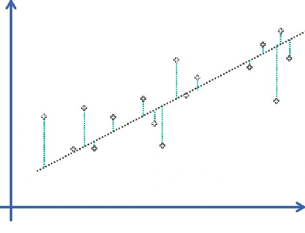
Error Function: $J=\sum_{n=1}^{m} (y-\hat y)^2$

Understanding support vectors

Unlike in the Ordinary Least Squares, the SVR model sets a threshold error allowance $\epsilon$ around the regression line such that all the data points within $\epsilon$ are not penalized for their error.

Image Source: Efficient Learning Machines Theories, Concepts, and Application for Engineers and System Designers by Mariette Awad and Rahul Khanna

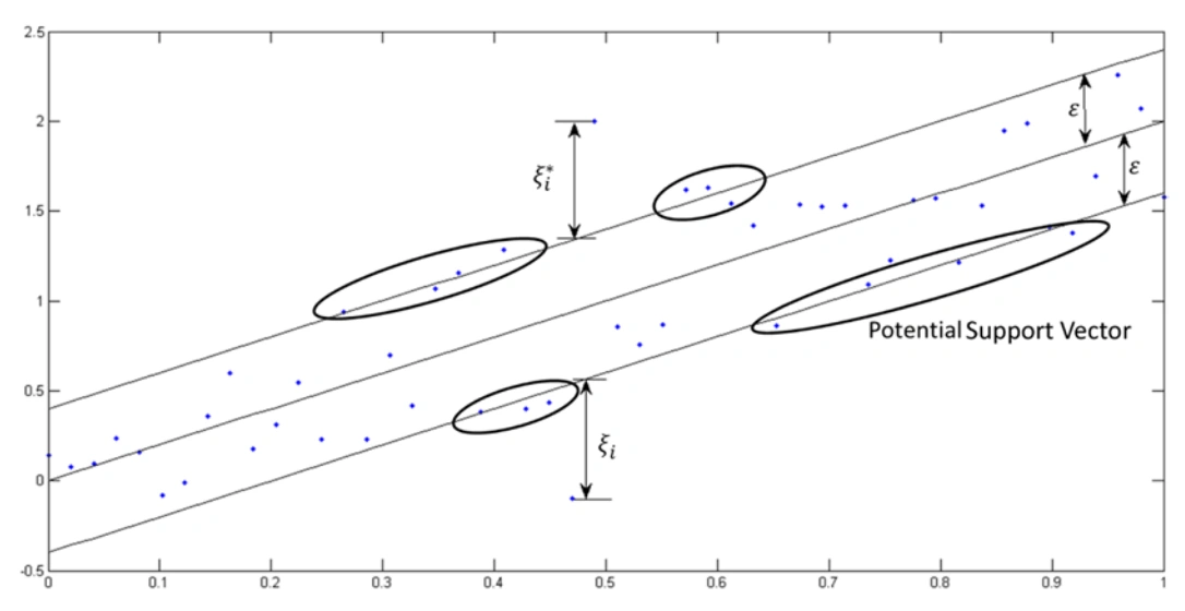
Therefore, the bound is error insensitive and is called $\epsilon$ – insensitive tube or simply $\epsilon$ – tube.

As we stated earlier, the distance between the regression line and the upper or lower bound is usually $\epsilon$ units. The $\epsilon$-tube is thus $2\epsilon$ units wide and symmetrical about the regression line.

Data points that fall outside the $\epsilon$-tube are penalized for their error:

• The error associated with the data point above $\epsilon$-tube is computed as the verticle distance between the datapoint and $\epsilon$-tube’s margin.
• If the data is below the tube, an error is the verticle distance between the $\epsilon$-tube’s lower bound and the datapoint.

We need to note that the error is taken from the tube’s margin and not the regression line.

Whenever a data point is above the tube’s margin, the deviation is denoted as $\zeta$ and $\zeta*$ when it is below. Both the $\zeta$ and $\zeta^*$ are called Slack Variables.

These points are the ones that dictate how the $\epsilon$-tube is created. They are thus called the Support Vector.

Formulating optimization problem

From the above discussion, we can formulate our optimization problem as follows:

• Since the slack variables denote the deviation of the data from the margin of the $\epsilon$-tube, they can only be zero or greater than zero.
• Since the error $\zeta^*$ is above the tolerance zone, they can only be greater than or equal to zero.

They will lead to the following constraints:

1. $\zeta^ \ \ge0$ for data points above the tolerance region.
2. $\zeta^*\ge0$ for the data points below the tolerance zone.

Since $\zeta$ values are taken as points in the outer region of the $\epsilon$ – insensitive tube, the deviation between the data point and the regression line must satisfy:

$y_i-(W^Tx + b) \ \le \ \epsilon + \zeta_i$, if the point is above the tube and,

$(W^Tx + b)-y_i \ \le \ \epsilon + \zeta^{*}_i$, if the point is below the tube.

Primal problem

Our objective is to ensure that $\sum(\zeta+\zeta^*_i)$, is minimal.

Therefore, our primal problem is:

$\frac{1}{2}||W||^2 \ + \ C\sum_{n=1}^{m} (\zeta+\zeta^*_i) \ \rightarrow$ minimize

Where $C$ is some constant that give weight on minimizing $\sum(\zeta+\zeta^*_i)$.

$\begin{aligned} &\textbf{Primal \ Problem}&\ \ Minimize \ w.r.t \ W \ , \ b: && Subjected \ to: \end{aligned}$

$\begin{aligned}
\frac{1}{2}||W||^2 \ + \ C\sum_{n=1}^{m} (\zeta+\zeta^_i) \ && y_i-(W^Tx + b) \ \le \ \epsilon + \zeta_i\
&& (W^Tx + b)-y_i \ \le \ \epsilon + \zeta^{}_i\
&&\zeta^ \ \ge0, \ \zeta^*\ge0
\end{aligned}
$

Above is a linear optimization problem. Here, Lagrangian multipliers would be appropriate for solving such a problem.

Since we clearly understood how the Support Vector Regression works and how to formulate its optimization problem, let’s now implement this algorithm in python.

Implementing SVR in Python

Data preprocessing

As in any other implementation, first, we get the necessary libraries in place. The code below imports these libraries:

# get the libraries
import numpy as np
import matplotlib.pyplot as plt
import pandas as pd

The dataset used in this session can be downloaded here.

# get the dataset
dataset = pd.read_csv('/content/drive/MyDrive/Position_Salaries.csv')
# our dataset in this implementation is small, and thus we can print it all instead of viewing only the end
print(dataset)

Output:

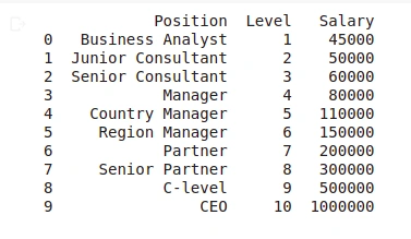
The above dataset contains ten instances. The significant feature in this dataset is the Level column. The Position column is just a description of the Level column, and therefore, it adds no value to our analysis.

Therefore, we will separate the dataset into a set of features and study variables.

As discussed above, we only have one feature in this dataset. Therefore, we carry out our feature-study variable separation as shown in the code below:

# split the data into featutes and target variable seperately
X_l = dataset.iloc[:, 1:-1].values # features set
y_p = dataset.iloc[:, -1].values # set of study variable

We can look at our feature set using the print() function.

print(X_l)

Output:

[[ 1]
 [ 2]
 [ 3]
 [ 4]
 [ 5]
 [ 6]
 [ 7]
 [ 8]
 [ 9]
 [10]]

From this output, it’s clear that the X_l variable is a 2D array. Similarly, we can have a look at the y_p variable:

print(y_p)

Output:

It’s seen from the output above that the y_p variable is a vector, i.e., a 1D array.

We need to note that the values of y_p are huge compared to x_l.

Therefore, if we implement a model on this data, the study variable will dominate the feature variable, such that its contribution to the model will be neglected.

Due to this, we will have to scale this study variable to the same range as the scaled study variable.

The challenge here is that the StandardScaler, the class we use to scale the data, takes in a 2D array; otherwise, it returns an error.

Due to this, we have to reshape our y_p variable from 1D to 2D. The code below does this for us:

y_p = y_p.reshape(-1,1)

Output:

[[  45000]
 [  50000]
 [  60000]
 [  80000]
 [ 110000]
 [ 150000]
 [ 200000]
 [ 300000]
 [ 500000]
 [1000000]]

From the above output, y_p was successfully reshaped into a 2D array.

Now, import the StandardScalar class and scale up the X_l and y_p variables separately as shown:

from sklearn.preprocessing import StandardScaler
StdS_X = StandardScaler()
StdS_y = StandardScaler()
X_l = StdS_X.fit_transform(X_l)
y_p = StdS_y.fit_transform(y_p)

Let’s simultaneously print and check if our two variables were scaled.

print("Scaled X_l:")
print(X_l)
print("Scaled y_p:")
print(y_p)

Output:

Scaled X_l:
[[-1.5666989 ]
 [-1.21854359]
 [-0.87038828]
 [-0.52223297]
 [-0.17407766]
 [ 0.17407766]
 [ 0.52223297]
 [ 0.87038828]
 [ 1.21854359]
 [ 1.5666989 ]]
Scaled y_p:
[[-0.72004253]
 [-0.70243757]
 [-0.66722767]
 [-0.59680786]
 [-0.49117815]
 [-0.35033854]
 [-0.17428902]
 [ 0.17781001]
 [ 0.88200808]
 [ 2.64250325]]

As we can see from the obtained output, both variables were scaled within the range -3 and +3.

Our data is now ready to implement our SVR model.

However, before we can do so, we will first visualize the data to know the nature of the SVR model that best fits it. So, let us create a scatter plot of our two variables.

plt.scatter(X_l, y_p, color = 'red') # plotting the training set
plt.title('Scatter Plot') # adding a tittle to our plot
plt.xlabel('Levels') # adds a label to the x-axis
plt.ylabel('Salary') # adds a label to the y-axis
plt.show() # prints

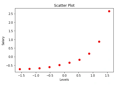
The plot shows a non-linear relationship between the Levels and Salary.

Due to this, we cannot use the linear SVR to model this data. Therefore, to capture this relationship better, we will use the SVR with the kernel functions.

Implementing SVR

To implement our model, first, we need to import it from the scikit-learn and create an object to itself.

Since we declared our data to be non-linear, we will pass it to a kernel called the Radial Basis function (RBF) kernel.

After declaring the kernel function, we will fit our data on the object. The following program performs these rules:

# import the model
from sklearn.svm import SVR
# create the model object
regressor = SVR(kernel = 'rbf')
# fit the model on the data
regressor.fit(X_l, y_p)

Since the model is now ready, we can use it and make predictions as shown:

A=regressor.predict(StdS_X.transform([[6.5]]))
print(A)

Output:

array([-0.27861589])

As we can see, the model prediction values are for the scaled study variable. But, the required value for the business is the output of the unscaled data. So, we need to get back to the real scale of the study variable.

To go back to the real study variable, we will write a program whose objective is to take the predicted values on the scaled range and transform them to the actual scale.

We do so by taking an inverse of the transformation on the study variable.

Note that the predicted values are returned in a 1D array.

However, as we can recall, we had reshaped our study variable from 1D to 2D array since the StandarScaler method takes in only 2D arrays.

So, for any predicted value to fit within such a new dimension of the study variable, it must be transformed from 1D to 2D; otherwise, we will get an error.

So, let’s implement these commands and get the required value:

# Convert A to 2D
A = A.reshape(-1,1)
print(A)

Output:

array([[-0.27861589]])

It is clear from the output above is a 2D array. Using the inverse_transform() function, we can convert it to an unscaled value in the original dataset as shown:

# Taking the inverse of the scaled value
A_pred = StdS_y.inverse_transform(A)
print(A_pred)

Output:

array([[170370.0204065]])

Here is the result, and it falls within the expected range.

However, if we were to run a polynomial regression on this data and predict the same values, we would have obtained the predicted values as 158862.45265155, which is only fixed on the curve.

With the Support Vector regression, this is not the case. So there is that allowance given to the model to make the best prediction.

Code optimization

We can optimize the above operation into a single line of code as below.

B_pred = StdS_y.inverse_transform(regressor.predict(StdS_X.transform([[6.5]])).reshape(-1,1))
print(B_pred)

Output:

array([[170370.0204065]])

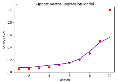
Since we now know how to implement and make predictions using the SVR model, the final thing we will do is to visualize our model.

The following code carries out this task:

# inverse the transformation to go back to the initial scale
plt.scatter(StdS_X.inverse_transform(X_l), StdS_y.inverse_transform(y_p), color = 'red')
plt.plot(StdS_X.inverse_transform(X_l), StdS_y.inverse_transform(regressor.predict(X_l).reshape(-1,1)), color = 'blue')
# add the title to the plot
plt.title('Support Vector Regression Model')
# label x axis
plt.xlabel('Position')
# label y axis
plt.ylabel('Salary Level')
# print the plot
plt.show()

Output:

Conclusion

In this article, we explored how Support Vector Regression works and formulated it’s optimization problem. Later, we learned to implement our model make predictions with it.

Finally, we learned to visualize the model. Thanks for reading to this end.

You can find the source code here.

Happy learning!

References

• Further reading on SVR

Peer Review Contributions by: Srishilesh P S