


The most typical strategy in machine learning is to divide a data set into training and validation sets. 70:30 or 80:20 could be the split ratio. It is the holdout method.
The problem with this strategy is that we don’t know if a high validation accuracy indicates a good model. What if the part of the data we utilized for validation turned out to be a success? Would our model still be accurate if we used a different section of the data set as a validation set? These are some questions that K-fold CV answers.
Prerequisites
To follow along with this tutorial, you need to have:
- The Wisconsin Breast Cancer data set. You can find it here.
- Google Colaboratory or Jupyter Notebook.
Introduction
K-fold cross-validation is a superior technique to validate the performance of our model. It evaluates the model using different chunks of the data set as the validation set.
We divide our data set into K-folds. K represents the number of folds into which you want to split your data. If we use 5-folds, the data set divides into five sections. In different iterations, one part becomes the validation set.
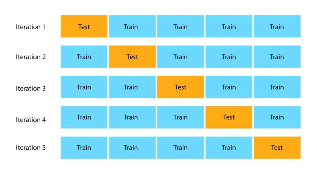
Image Source: Great Learning Blog
In the first iteration, we use the first part of the data for validation. As illustrated in the image above, we use the other parts of the data set for training.
Data preprocessing
We import all the relevant libraries for the project and load the data set.
# import relevant libraries
import numpy as np
import pandas as pd
import matplotlib.pyplot as plt
import seaborn as sns
from sklearn.metrics import f1_score
%matplotlib inline

# load dataset
dataset = pd.read_csv('breast_cancer_data.csv')
dataset
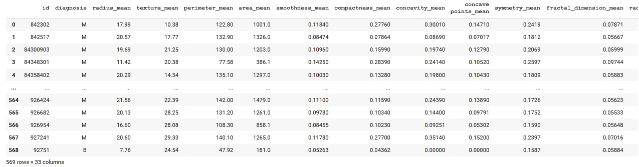
The target variable is the diagnosis column. It has an index of 1. The features are all the columns except the id, diagnosis and Unnamed: 32 columns.
# Separate features and target variable
X = dataset.iloc[:, 2:-1].values
y = dataset. iloc [:, 1].values
print("Matrix of features", X, sep='\n')
print("--------------------------------------------------")
print("Target Variable", y, sep='\n')
Output:
    Matrix of features
    [[1.799e+01 1.038e+01 1.228e+02 ... 2.654e-01 4.601e-01 1.189e-01]
     [2.057e+01 1.777e+01 1.329e+02 ... 1.860e-01 2.750e-01 8.902e-02]
     [1.969e+01 2.125e+01 1.300e+02 ... 2.430e-01 3.613e-01 8.758e-02]
     ...
     [1.660e+01 2.808e+01 1.083e+02 ... 1.418e-01 2.218e-01 7.820e-02]
     [2.060e+01 2.933e+01 1.401e+02 ... 2.650e-01 4.087e-01 1.240e-01]
     [7.760e+00 2.454e+01 4.792e+01 ... 0.000e+00 2.871e-01 7.039e-02]]
    --------------------------------------------------
    Target Variable
    ['M' 'M' 'M' 'M' 'M' 'M' 'M' 'M' 'M' 'M' 'M' 'M' 'M' 'M' 'M' 'M' 'M' 'M'
     'M' 'B' 'B' 'B' 'M' 'M' 'M' 'M' 'M' 'M' 'M' 'M' 'M' 'M' 'M' 'M' 'M' 'M'
     'M' 'B' 'M' 'M' 'M' 'M' 'M' 'M' 'M' 'M' 'B' 'M' 'B' 'B' 'B' 'B' 'B' 'M'
     'M' 'B' 'M' 'M' 'B' 'B' 'B' 'B' 'M' 'B' 'M' 'M' 'B' 'B' 'B' 'B' 'M' 'B'
     'M' 'M' 'B' 'M' 'B' 'M' 'M' 'B' 'B' 'B' 'M' 'M' 'B' 'M' 'M' 'M' 'B' 'B'
     'B' 'M' 'B' 'B' 'M' 'M' 'B' 'B' 'B' 'M' 'M' 'B' 'B' 'B' 'B' 'M' 'B' 'B'
     'M' 'B' 'B' 'B' 'B' 'B' 'B' 'B' 'B' 'M' 'M' 'M' 'B' 'M' 'M' 'B' 'B' 'B'
     'M' 'M' 'B' 'M' 'B' 'M' 'M' 'B' 'M' 'M' 'B' 'B' 'M' 'B' 'B' 'M' 'B' 'B'
     'B' 'B' 'M' 'B' 'B' 'B' 'B' 'B' 'B' 'B' 'B' 'B' 'M' 'B' 'B' 'B' 'B' 'M'
     'M' 'B' 'M' 'B' 'B' 'M' 'M' 'B' 'B' 'M' 'M' 'B' 'B' 'B' 'B' 'M' 'B' 'B'
     'M' 'M' 'M' 'B' 'M' 'B' 'M' 'B' 'B' 'B' 'M' 'B' 'B' 'M' 'M' 'B' 'M' 'M'
     'M' 'M' 'B' 'M' 'M' 'M' 'B' 'M' 'B' 'M' 'B' 'B' 'M' 'B' 'M' 'M' 'M' 'M'
     'B' 'B' 'M' 'M' 'B' 'B' 'B' 'M' 'B' 'B' 'B' 'B' 'B' 'M' 'M' 'B' 'B' 'M'
     'B' 'B' 'M' 'M' 'B' 'M' 'B' 'B' 'B' 'B' 'M' 'B' 'B' 'B' 'B' 'B' 'M' 'B'
     'M' 'M' 'M' 'M' 'M' 'M' 'M' 'M' 'M' 'M' 'M' 'M' 'M' 'M' 'B' 'B' 'B' 'B'
     'B' 'B' 'M' 'B' 'M' 'B' 'B' 'M' 'B' 'B' 'M' 'B' 'M' 'M' 'B' 'B' 'B' 'B'
     'B' 'B' 'B' 'B' 'B' 'B' 'B' 'B' 'B' 'M' 'B' 'B' 'M' 'B' 'M' 'B' 'B' 'B'
     'B' 'B' 'B' 'B' 'B' 'B' 'B' 'B' 'B' 'B' 'B' 'M' 'B' 'B' 'B' 'M' 'B' 'M'
     'B' 'B' 'B' 'B' 'M' 'M' 'M' 'B' 'B' 'B' 'B' 'M' 'B' 'M' 'B' 'M' 'B' 'B'
     'B' 'M' 'B' 'B' 'B' 'B' 'B' 'B' 'B' 'M' 'M' 'M' 'B' 'B' 'B' 'B' 'B' 'B'
     'B' 'B' 'B' 'B' 'B' 'M' 'M' 'B' 'M' 'M' 'M' 'B' 'M' 'M' 'B' 'B' 'B' 'B'
     'B' 'M' 'B' 'B' 'B' 'B' 'B' 'M' 'B' 'B' 'B' 'M' 'B' 'B' 'M' 'M' 'B' 'B'
     'B' 'B' 'B' 'B' 'M' 'B' 'B' 'B' 'B' 'B' 'B' 'B' 'M' 'B' 'B' 'B' 'B' 'B'
     'M' 'B' 'B' 'M' 'B' 'B' 'B' 'B' 'B' 'B' 'B' 'B' 'B' 'B' 'B' 'B' 'M' 'B'
     'M' 'M' 'B' 'M' 'B' 'B' 'B' 'B' 'B' 'M' 'B' 'B' 'M' 'B' 'M' 'B' 'B' 'M'
     'B' 'M' 'B' 'B' 'B' 'B' 'B' 'B' 'B' 'B' 'M' 'M' 'B' 'B' 'B' 'B' 'B' 'B'
     'M' 'B' 'B' 'B' 'B' 'B' 'B' 'B' 'B' 'B' 'B' 'M' 'B' 'B' 'B' 'B' 'B' 'B'
     'B' 'M' 'B' 'M' 'B' 'B' 'M' 'B' 'B' 'B' 'B' 'B' 'M' 'M' 'B' 'M' 'B' 'M'
     'B' 'B' 'B' 'B' 'B' 'M' 'B' 'B' 'M' 'B' 'M' 'B' 'M' 'M' 'B' 'B' 'B' 'M'
     'B' 'B' 'B' 'B' 'B' 'B' 'B' 'B' 'B' 'B' 'B' 'M' 'B' 'M' 'M' 'B' 'B' 'B'
     'B' 'B' 'B' 'B' 'B' 'B' 'B' 'B' 'B' 'B' 'B' 'B' 'B' 'B' 'B' 'B' 'B' 'B'
     'B' 'B' 'B' 'B' 'M' 'M' 'M' 'M' 'M' 'M' 'B']
The target variable contains strings, we must change the strings to numbers.
# Label Encode the target variable
from sklearn.preprocessing import LabelEncoder
label_encoder = LabelEncoder()
encoded_y = label_encoder.fit_transform(y)
label_encoder_name_mapping = dict(zip(label_encoder.classes_,
                                         label_encoder.transform(label_encoder.classes_)))
print("Mapping of Label Encoded Classes", label_encoder_name_mapping, sep="\n")
print("Label Encoded Target Variable", encoded_y, sep="\n")
Output:
    Mapping of Label Encoded Classes
    {'B': 0, 'M': 1}
    Label Encoded Target Variable
    [1 1 1 1 1 1 1 1 1 1 1 1 1 1 1 1 1 1 1 0 0 0 1 1 1 1 1 1 1 1 1 1 1 1 1 1 1
     0 1 1 1 1 1 1 1 1 0 1 0 0 0 0 0 1 1 0 1 1 0 0 0 0 1 0 1 1 0 0 0 0 1 0 1 1
     0 1 0 1 1 0 0 0 1 1 0 1 1 1 0 0 0 1 0 0 1 1 0 0 0 1 1 0 0 0 0 1 0 0 1 0 0
     0 0 0 0 0 0 1 1 1 0 1 1 0 0 0 1 1 0 1 0 1 1 0 1 1 0 0 1 0 0 1 0 0 0 0 1 0
     0 0 0 0 0 0 0 0 1 0 0 0 0 1 1 0 1 0 0 1 1 0 0 1 1 0 0 0 0 1 0 0 1 1 1 0 1
     0 1 0 0 0 1 0 0 1 1 0 1 1 1 1 0 1 1 1 0 1 0 1 0 0 1 0 1 1 1 1 0 0 1 1 0 0
     0 1 0 0 0 0 0 1 1 0 0 1 0 0 1 1 0 1 0 0 0 0 1 0 0 0 0 0 1 0 1 1 1 1 1 1 1
     1 1 1 1 1 1 1 0 0 0 0 0 0 1 0 1 0 0 1 0 0 1 0 1 1 0 0 0 0 0 0 0 0 0 0 0 0
     0 1 0 0 1 0 1 0 0 0 0 0 0 0 0 0 0 0 0 0 0 1 0 0 0 1 0 1 0 0 0 0 1 1 1 0 0
     0 0 1 0 1 0 1 0 0 0 1 0 0 0 0 0 0 0 1 1 1 0 0 0 0 0 0 0 0 0 0 0 1 1 0 1 1
     1 0 1 1 0 0 0 0 0 1 0 0 0 0 0 1 0 0 0 1 0 0 1 1 0 0 0 0 0 0 1 0 0 0 0 0 0
     0 1 0 0 0 0 0 1 0 0 1 0 0 0 0 0 0 0 0 0 0 0 0 1 0 1 1 0 1 0 0 0 0 0 1 0 0
     1 0 1 0 0 1 0 1 0 0 0 0 0 0 0 0 1 1 0 0 0 0 0 0 1 0 0 0 0 0 0 0 0 0 0 1 0
     0 0 0 0 0 0 1 0 1 0 0 1 0 0 0 0 0 1 1 0 1 0 1 0 0 0 0 0 1 0 0 1 0 1 0 1 1
     0 0 0 1 0 0 0 0 0 0 0 0 0 0 0 1 0 1 1 0 0 0 0 0 0 0 0 0 0 0 0 0 0 0 0 0 0
     0 0 0 0 0 0 0 1 1 1 1 1 1 0]
The number 0 represents benign, while 1 represents malignant.
5-Fold cross-validation
We use the cross_validate function from the Scikit-Learn library’s model_selection module.
# K-Fold Cross-Validation
from sklearn.model_selection import cross_validate
def cross_validation(model, _X, _y, _cv=5):
      '''Function to perform 5 Folds Cross-Validation
       Parameters
       ----------
      model: Python Class, default=None
              This is the machine learning algorithm to be used for training.
      _X: array
           This is the matrix of features.
      _y: array
           This is the target variable.
      _cv: int, default=5
          Determines the number of folds for cross-validation.
       Returns
       -------
       The function returns a dictionary containing the metrics 'accuracy', 'precision',
       'recall', 'f1' for both training set and validation set.
      '''
      _scoring = ['accuracy', 'precision', 'recall', 'f1']
      results = cross_validate(estimator=model,
                               X=_X,
                               y=_y,
                               cv=_cv,
                               scoring=_scoring,
                               return_train_score=True)

      return {"Training Accuracy scores": results['train_accuracy'],
              "Mean Training Accuracy": results['train_accuracy'].mean()*100,
              "Training Precision scores": results['train_precision'],
              "Mean Training Precision": results['train_precision'].mean(),
              "Training Recall scores": results['train_recall'],
              "Mean Training Recall": results['train_recall'].mean(),
              "Training F1 scores": results['train_f1'],
              "Mean Training F1 Score": results['train_f1'].mean(),
              "Validation Accuracy scores": results['test_accuracy'],
              "Mean Validation Accuracy": results['test_accuracy'].mean()*100,
              "Validation Precision scores": results['test_precision'],
              "Mean Validation Precision": results['test_precision'].mean(),
              "Validation Recall scores": results['test_recall'],
              "Mean Validation Recall": results['test_recall'].mean(),
              "Validation F1 scores": results['test_f1'],
              "Mean Validation F1 Score": results['test_f1'].mean()
              }
The custom cross_validation function in the code above will perform 5-fold cross-validation. It returns the results of the metrics specified above.
The estimator parameter of the cross_validate function receives the algorithm we want to use for training. The parameter X takes the matrix of features. The parameter y takes the target variable. The parameter scoring takes the metrics we want to use for evaluation. We pass a list containing metrics we want to use to check our model.
For this guide, we will use accuracy, precision, recall, and f1 score. Setting the return_train_score to True will give us the training results.
We create a function to visualize the training and validation results in each fold. The function will display a grouped bar chart.
# Grouped Bar Chart for both training and validation data
def plot_result(x_label, y_label, plot_title, train_data, val_data):
        '''Function to plot a grouped bar chart showing the training and validation
          results of the ML model in each fold after applying K-fold cross-validation.
         Parameters
         ----------
         x_label: str,
            Name of the algorithm used for training e.g 'Decision Tree'

         y_label: str,
            Name of metric being visualized e.g 'Accuracy'
         plot_title: str,
            This is the title of the plot e.g 'Accuracy Plot'

         train_result: list, array
            This is the list containing either training precision, accuracy, or f1 score.

         val_result: list, array
            This is the list containing either validation precision, accuracy, or f1 score.
         Returns
         -------
         The function returns a Grouped Barchart showing the training and validation result
         in each fold.
        '''

        # Set size of plot
        plt.figure(figsize=(12,6))
        labels = ["1st Fold", "2nd Fold", "3rd Fold", "4th Fold", "5th Fold"]
        X_axis = np.arange(len(labels))
        ax = plt.gca()
        plt.ylim(0.40000, 1)
        plt.bar(X_axis-0.2, train_data, 0.4, color='blue', label='Training')
        plt.bar(X_axis+0.2, val_data, 0.4, color='red', label='Validation')
        plt.title(plot_title, fontsize=30)
        plt.xticks(X_axis, labels)
        plt.xlabel(x_label, fontsize=14)
        plt.ylabel(y_label, fontsize=14)
        plt.legend()
        plt.grid(True)
        plt.show()
Model training
Now we can train our machine learning algorithm. We will use a decision tree algorithm. We import the DecisionTreeClassifier from the tree module of the Scikit-Learn library. We also invoke the cross_validation function we created earlier to perform 5-fold cross-validation.
from sklearn.tree import DecisionTreeClassifier
decision_tree_model = DecisionTreeClassifier(criterion="entropy",
                                     random_state=0)
decision_tree_result = cross_validation(decision_tree_model, X, encoded_y, 5)
print(decision_tree_result)
Output:
{'Training Accuracy scores': array([1., 1., 1., 1., 1.]),
'Mean Training Accuracy': 100.0,
'Training Precision scores': array([1., 1., 1., 1., 1.]),
'Mean Training Precision': 1.0,
'Training Recall scores': array([1., 1., 1., 1., 1.]),
'Mean Training Recall': 1.0,
'Training F1 scores': array([1., 1., 1., 1., 1.]),
'Mean Training F1 Score': 1.0,
'Validation Accuracy scores': array([0.9122807 , 0.92105263, 0.94736842, 0.94736842, 0.94690265]),
'Mean Validation Accuracy': 93.49945660611706,
'Validation Precision scores': array([0.92307692, 0.94736842, 0.90909091, 0.89130435, 0.89130435]),
'Mean Validation Precision': 0.9124289897745275,
'Validation Recall scores': array([0.8372093 , 0.8372093 , 0.95238095, 0.97619048, 0.97619048]),
'Mean Validation Recall': 0.9158361018826134,
'Validation F1 scores': array([0.87804878, 0.88888889, 0.93023256, 0.93181818, 0.93181818]),
'Mean Validation F1 Score': 0.9121613182305184}
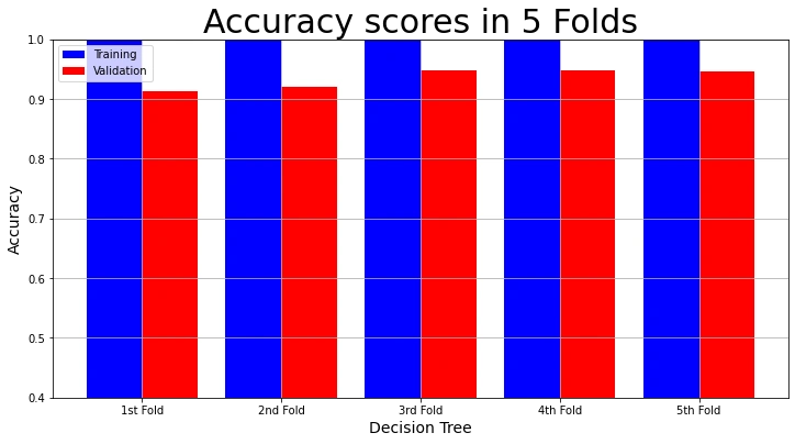
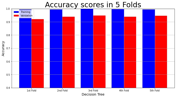
To understand the results better, we can visualize them. We use the plot_result function we created earlier. We start by visualizing the training accuracy and validation accuracy in each fold.
# Plot Accuracy Result
model_name = "Decision Tree"
plot_result(model_name,
            "Accuracy",
            "Accuracy scores in 5 Folds",
            decision_tree_result["Training Accuracy scores"],
            decision_tree_result["Validation Accuracy scores"])
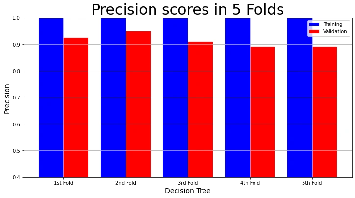
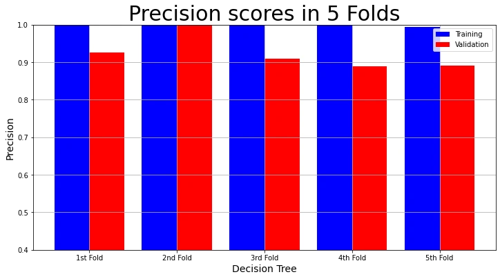
We can also visualize the training precision and validation precision in each fold.
# Plot Precision Result
plot_result(model_name,
            "Precision",
            "Precision scores in 5 Folds",
            decision_tree_result["Training Precision scores"],
            decision_tree_result["Validation Precision scores"])
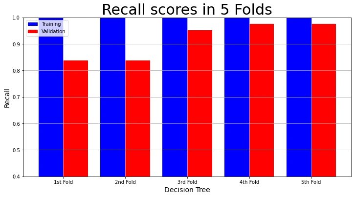
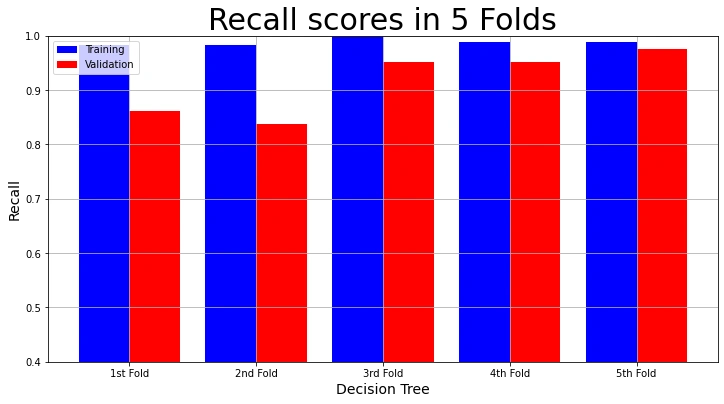
Let us visualize the training recall and validation recall in each fold.
# Plot Recall Result
plot_result(model_name,
            "Recall",
            "Recall scores in 5 Folds",
            decision_tree_result["Training Recall scores"],
            decision_tree_result["Validation Recall scores"])
Finally, we visualize the training f1 score and validation f1 score in each fold.
# Plot F1-Score Result
plot_result(model_name,
            "F1",
            "F1 Scores in 5 Folds",
            decision_tree_result["Training F1 scores"],
            decision_tree_result["Validation F1 scores"])
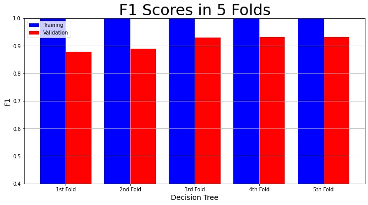
The visualizations show that the training accuracy, precision, recall, and f1 scores in each fold are 100%. But the validation accuracy, precision, recall and f1 scores are not as high. We call this over-fitting. The model performs admirably on the training data. But not so much on the validation set.
Visualizing your results like this can help you see if your model is over-fitting. We adjust the min_samples_split hyper-parameter in the decision tree algorithm. It will fix the over-fitting problem. The default value of the min_samples_split parameter is 2. We increase the value to 5.
decision_tree_model_2 = DecisionTreeClassifier(criterion="entropy",
                                               min_samples_split=5,
                                               random_state=0)
decision_tree_result_2 = cross_validation(decision_tree_model_2, X, encoded_y, 5)
print(decision_tree_result_2)
Output:
{'Training Accuracy scores': array([0.99340659, 0.99340659, 1.        , 0.9956044 , 0.99342105]),
'Mean Training Accuracy': 99.51677270098322,
'Training Precision scores': array([1.        , 1.        , 1.        , 1.        , 0.99408284]),
'Mean Training Precision': 0.9988165680473372,
'Training Recall scores': array([0.98224852, 0.98224852, 1.        , 0.98823529, 0.98823529]),
'Mean Training Recall': 0.9881935259310826,
'Training F1 scores': array([0.99104478, 0.99104478, 1.        , 0.99408284, 0.99115044]),
'Mean Training F1 Score': 0.9934645669906736,
'Validation Accuracy scores': array([0.92105263, 0.93859649, 0.94736842, 0.93859649, 0.94690265]),
'Mean Validation Accuracy': 93.85033379909953,
'Validation Precision scores': array([0.925     , 1.        , 0.90909091, 0.88888889, 0.89130435]),
'Mean Validation Precision': 0.9228568291611768,
'Validation Recall scores': array([0.86046512, 0.8372093 , 0.95238095, 0.95238095, 0.97619048]),
'Mean Validation Recall': 0.9157253599114064,
'Validation F1 scores': array([0.89156627, 0.91139241, 0.93023256, 0.91954023, 0.93181818]),
'Mean Validation F1 Score': 0.9169099279932611}
Let us visualize the results of the second model.
The training accuracy and validation accuracy in each fold:
# Plot Accuracy Result
plot_result(model_name,
            "Accuracy",
            "Accuracy scores in 5 Folds",
            decision_tree_result_2["Training Accuracy scores"],
            decision_tree_result_2["Validation Accuracy scores"])
The training precision and validation precision in each fold:
# Plot Precision Result
plot_result(model_name,
            "Precision",
            "Precision scores in 5 Folds",
            decision_tree_result_2["Training Precision scores"],
            decision_tree_result_2["Validation Precision scores"])
The training recall and validation recall in each fold:
# Plot Recall Result
plot_result(model_name,
            "Recall",
            "Recall scores in 5 Folds",
            decision_tree_result_2["Training Recall scores"],
            decision_tree_result_2["Validation Recall scores"])
The training f1 score and validation f1 score in each fold:
# Plot F1-Score Result
plot_result(model_name,
            "F1",
            "F1 Scores in 5 Folds",
            decision_tree_result_2["Training F1 scores"],
            decision_tree_result_2["Validation F1 scores"])
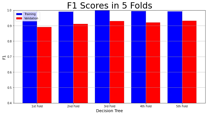
We can see that the validation results of the second model in each fold are better. It has a mean validation accuracy of 93.85% and a mean validation f1 score of 91.69%. You can find the GitHub repo for this project here.
Conclusion
When training a model on a small data set, the K-fold cross-validation technique comes in handy. You may not need to use K-fold cross-validation if your data collection is huge. The reason is you have enough records in your validation set to check the machine learning model. It takes a lot of time to use K-fold cross-validation on a large data collection.
Finally, using more folds to check your model consumes more computing resources. The higher the value of K, the longer it will take to train the model. If K=5, the model trains five times using five different folds as the validation set. If K=10, the model trains ten times.


Comments: