Hyperparameter Tuning in Decision Trees and Random Forests

After years of hard work, we have reached a stage where we use computers to analyze millions of data points and provide insights that even the human eye could not catch.

But our Machine Learning model is only as good as its accuracy on unseen data, i.e., “how well our model generalizes”. In this article, we’ll solve a binary classification problem, using a Decision Tree classifier and Random Forest to solve the over-fitting problem by tuning their hyper-parameters and comparing results.

Before we begin, you should have some working knowledge of Python and some basic understanding of Machine Learning. If you’re new to Decision Trees entirely, you can still go ahead and begin reading. Irrespective, let’s begin with a brief introduction to Machine Learning.

Machine Learning

Machine Learning is the practice of emulating a human being’s learning and reasoning ability, along with the continuous enhancement of results with every additional data input. This is also called continual learning. Any new input entered will contribute to the accuracy of the algorithm. Hence, they learn from experience like the human brain.

Based on these algorithms, we create a model and train it over a set of data to recognize certain patterns.

Dataset

This article will use the heart disease prediction dataset. It consists of almost 70,000 rows of data points with 12 columns, featuring a person’s medical record. All the necessary preprocessing on this dataset has been done priorly. You can find the code hosted on Jovian here.

Now, let’s get to the models in hand.

Decision Tree

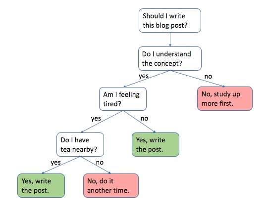
Decision Trees are powerful machine learning algorithms capable of performing regression and classification tasks. To understand a decision tree, let’s look at an inverted tree-like structure (like that of a family tree). We start at the root of the tree that contains our training data. At the root, we split our dataset into distinguished leaf nodes, following certain conditions like using an if/else loop.

Image Source: Jeremy Jordan

These splitting criteria are carefully calculated using a splitting technique. We’ll understand a few of them in the working of a decision tree section.

So all-in-all, decision trees are a hierarchical series of binary decisions, and the antecedent nodes are simply the best split for the available training data at each level of our decision tree.

Working of a Decision Tree

To understand how our model splits our training data and grows into a decision tree, we need to understand some fundamental splitting parameters that it uses to define those conditions, like Gini Index, Entropy, Information Gain, etc.

Gini Score/ Gini Index

Every Machine Learning model has a loss function or a cost function, whose objective is to minimize the cost, i.e., the tentative distance between the predicted value and actual value. (For classification problems, probabilities of predicted class are used). Gini Index is the cost/loss function that is used by decision trees to choose which feature will be used for splitting the data, and at what point the column should be split.

$$Lower\space Gini\space Score \iff Lower\space Cost \iff Good\space Split$$
⭐️ A perfect split with only two features and two classes has Gini Index = 0.

Entropy

Entropy measures the randomness or disorders in a system. In terms of data, we can define it as the randomness in the information we are processing. The higher the randomness, the higher the entropy. Hence, harder to conclude from that information. Mathematically, we calculate entropy as:

$$entropy = - \sum_{i = 1}^{k}{P(value_i).{log_2}(P(value_i))}$$

Information gain

Information gain (IG) measures the amount of information provided by a given feature or attribute about a particular target class. While creating a decision tree, our goal is to find the attribute having the highest Information Gain, and conversely, the lowest entropy. Mathematically, it is calculated as the difference of the initial and final entropy. For example:

$$I_{gain} = Entropy_{before\space split} - Entropy_{after\space split}$$

This is how information gain and entropy are used to improve the quality of splitting.

If we use Information Gain as a criterion, we assume that our attributes are categorical, and as per Gini index, we assume that our attributes are continuous. For our dataset, we will work with Gini Index.

Working:

• While training, our decision tree model evaluates all possible splits across all possible columns and picks the split with the lowest Gini Score.
• With the first split, all the data according to a specific condition falls towards either the left or the right of the root node.
• Now, for each side of training data under the root node, all possible splits are calculated again and the split with the lowest Gini Index is chosen. The process repeats for both left and right sides till we reach the terminating nodes representing a class in the target column.

Media Source

This way, our decision tree grows iteratively, layer by layer.

Training and visualizing Decision Trees

from sklearn.tree import DecisionTreeClassifier
model2 = DecisionTreeClassifier(random_state=42)
model2.fit(train_inputs, train_targets)

We should split the training data into train, validation, and test sets, which is another crucial step in preprocessing.

For visualization, make sure to import all the necessary libraries like matplotlib, seaborn, etc. To visualize a decision tree, we use the plot_tree function from sklearn.

#Visualizing a Decision Tree
from sklearn.tree import plot_tree, export_text
plt.figure(figsize =(80,20))

plot_tree(model2, feature_names=train_inputs.columns, max_depth=2, filled=True);

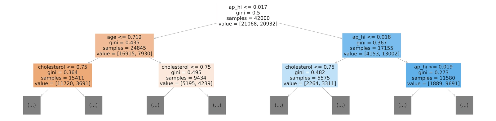
You can create the tree to whatsoever depth using the max_depth attribute, only two layers of the output are shown above. Let’s break the blocks in the above visualization:

• ap_hi≤0.017: Is the condition on which the data is being split. (where ap_hi is the column name).
• Gini: Is the Gini Index. Although the root node has a Gini index of 0.5, which is not so great, we can imagine what the other Gini scores would have looked like.
• Samples: The number of data rows before the split.
• Values=[x,y]: Provides the split rows of training data into the following leaf nodes. Since we are doing binary classification, there are only two values.

Evaluation, overfitting, and regularization

Now that we’ve trained our model, let’s calculate its accuracy on training and validation sets. We’ve evaluated our model using the accuracy score and confusion matrix. Let’s not get into it, but you can choose any evaluation metrics you’re comfortable with.

from sklearn.metrics import accuracy_score, confusion_matrix

The following are the results with basic implementation of Decision Trees:

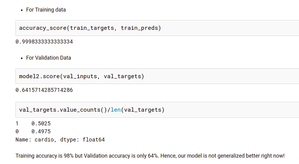
It is axiomatic in the results above that our model is not performing well on data it has not been trained upon, but giving incredulous results on training data. This simple phenomenon is called Overfitting. This is happening because our model has memorized all the training examples.

Regularization: The process of reducing overfitting. Regularization is done differently in regression models. But for a decision tree classifier, we will perform regularization by providing additional arguments accepted by DecisionTreeClassifier. These arguments provided by us to revamp our model are called HyperParameters.

Hyperparameter and parameters: Parameters are the model features that the model learns from the data. Whereas, Hyperparameters are arguments accepted by a model-making function and can be modified to reduce overfitting, leading to a better generalization of the model.

Hyperparameter tuning in Decision Trees

This process of calibrating our model by finding the right hyperparameters to generalize our model is called Hyperparameter Tuning. We will look at a few of these hyperparameters:

a. Max Depth

This argument represents the maximum depth of a tree. If not specified, the tree is expanded until the last leaf nodes contain a single value. Hence by reducing this meter, we can preclude the tree from learning all training samples thereby, preventing over-fitting.

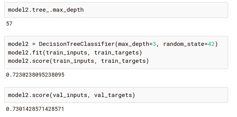
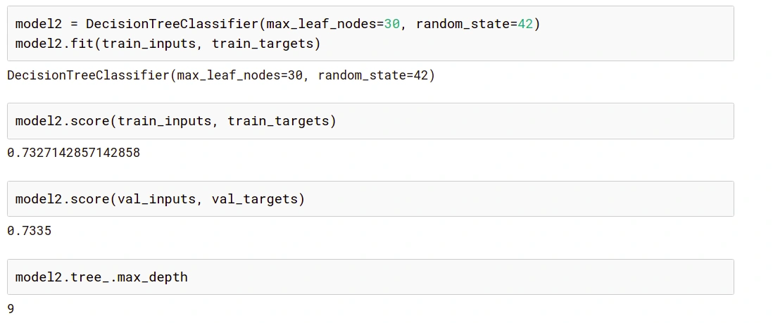
We can check the current maximum depth of our decision tree with model2.tree_.max_depth. It is evident that even though the training accuracy has reduced, the validation accuracy has improved.

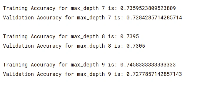
Since we are not sure what depth our ideal model would have, we can run a for loop from a range of numbers to find out. You can see below, we’ve used this basic for loop to print the training and validation accuracy of our model across the range 1–21.

for max_d in range(1,21):
  model = DecisionTreeClassifier(max_depth=max_d, random_state=42)
  model.fit(train_inputs, train_targets)
  print('The Training Accuracy for max_depth {} is:'.format(max_d), model.score(train_inputs, train_targets))
  print('The Validation Accuracy for max_depth {} is:'.format(max_d), model.score(val_inputs,val_targets))
  print('')

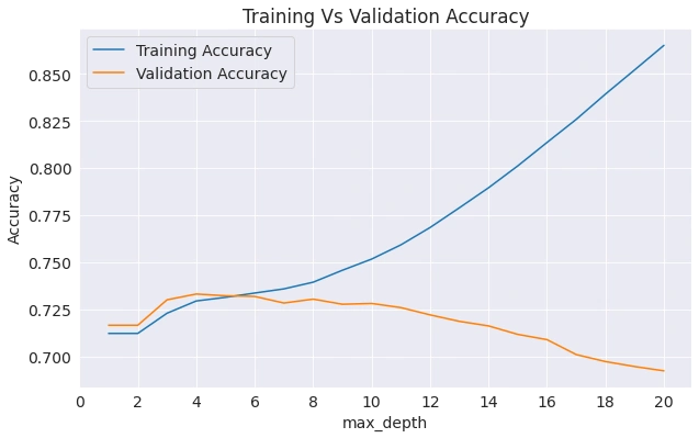
By carefully looking at the results, we can find the max_depth value where the validation accuracy starts decreasing, and the training accuracy starts mounting inordinately.

As you can see above, in our case, the pertinent max_depth=8.

To understand better, we can plot the resulting accuracies as shown below. You can see the curve where the model begins to overfit.

b. Max leaf nodes

As the name suggests, this hyperparameter caps the number of leaf nodes in a decision tree. It will allow the branches of a tree to have varying depths, another way to control the model’s complexity.

How?: In this case, the model will not find the best split layer by layer. Instead, it will look at all the possible splits (left and right) and only split the node with the lowest Gini Value, irrespective of the level.

To change the number of maximum leaf nodes, we use, max_leaf_nodes.

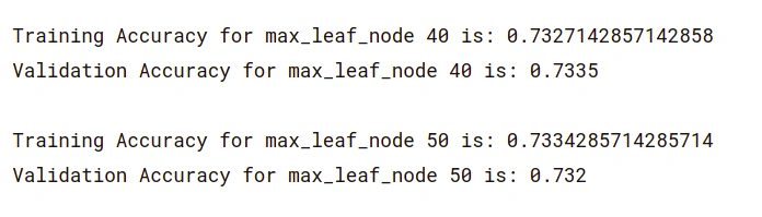
Here is the result of our model’s training and validation accuracy at different values of max_leaf_node hyperparameter:

While tuning the hyper-parameters of a single decision tree is giving us some improvement, a stratagem would be to merge the results of diverse decision trees (like a forest) with moderately different parameters. It is what we will understand in a random forest. So let’s practice some other hyper-parameters like max_features, min_samples_split, etc., under random forests.

Random Forests

Random forests are supervised machine learning models that train multiple decision trees and integrate the results by averaging them. Each decision tree makes various kinds of errors, and upon averaging their results, many of these errors are counterbalanced. This general practice of combining the results of many models is called “Emsembling technique”, or very famously said, “Wisdom of the crowd”.

Image Source

from sklearn.ensemble import RandomForestClassifier
model3 = RandomForestClassifier(random_state = 24, n_jobs = -1)
model3.fit(train_inputs, train_targets)

Note: In the code above, the function of the argument n_jobs = -1 is to train multiple decision trees parallelly.

We can access individual decision trees using model.estimators. We can visualize each decision tree inside a random forest separately as we visualized a decision tree prior in the article.

Hyperparameter Tuning in Random Forests

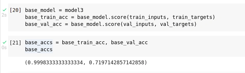
To compare results, we can create a base model without any hyperparameters.

The max_leaf_nodes and max_depth arguments above are directly passed on to each decision tree. They control the depth and maximum nodes of each tree, respectively. Now let’s explore some other hyperparameters:

c. n_estimators

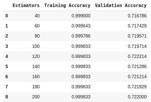
This argument limits the number of decision trees in random forests. By default, its value is calibrated to 100, but in the case of larger datasets, 100 can prove to be a meager quantity. Hence, it’s better to try a higher number of estimators.

model = RandomForestClassifier(random_state=42, n_jobs=-1, n_estimators=10)
model.fit(train_inputs, train_targets)

Typically, n_estimators should be kept minimal. For example, in our model, the validation accuracy of 100 and 200 estimators is approximately the same. So in such cases, we will stick to the lower number of estimators.

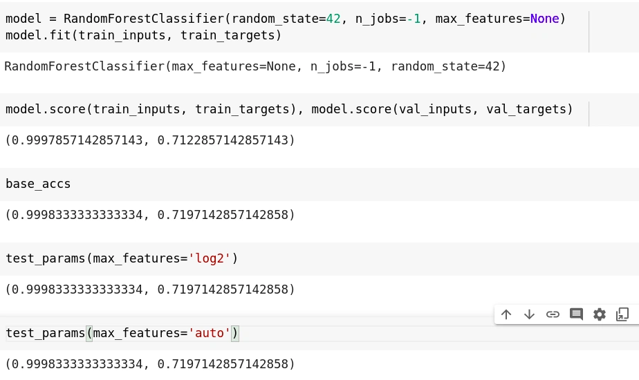
d. max_features

Instead of taking all the features into account for a split, we can circumscribe that only a few columns be selected.

Each time a split occurs, the model will only consider a fraction of columns. This will help to generalize our random forest model. If every time, all the features are considered at all splits, the random forest model will contain identical trees.

Hence, max_features will help make each tree in the forest different. The default value for this is “auto”, which is equivalent to the square root of the no. of features. Other values are: “log2”, “sqrt” and None. We got approximately the same results for all cases in our model.

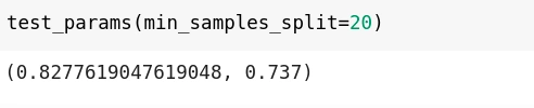
e. min_samples_split

Minimum samples split decides or hold the value for the minimum number of samples necessary to split a nonterminal node. By default, the decision tree tries to split every node that has two or more rows of data inside it. This can again cause memorization of training data, resulting in a lesser generalized model.

Larger values can restrict a model from learning relations that could be extremely specific to a particular row. But again, much-exceeded values for the same will lead to under-fitting the model. Therefore, depending upon the model requirements and chosen data, you can tune the values for min_samples_split.

The test_params function used above has the following code. It’s used to test different hyper parameters and returns the training and validation accuracy.

def test_params(**params):
    model = RandomForestClassifier(n_jobs=-1, random_state=24, **params).fit(X_train, train_targets)
    return model.score(X_train, train_targets), model.score(X_val, val_targets)

f. min_samples_leaf

Minimum sample leaf may sound like minimum sample split and is somewhat similar too. But in this case, we are talking about the minimum number of samples required to be left at the leaf node. A split will only be considered if there are at least min_samples_leaf samples on the left and right branches.

g. min_impurity_decrease

This argument is used to supervise the threshold for splitting nodes, i.e., a split will only take place if it reduces the Gini Impurity, greater than or equal to the min_impurity_decrease value. Its default value is 0, and we can modify it to decrease over-fitting. Since the number of features in our dataset is limited, there was no need to try this particular hyperparameter.

Some default hyperparameters used in random forests are Bootstrapping.

Bootstrap

By default, Random Forest does not use the whole dataset for fitting each decision tree. Instead, while creating decision trees, random rows of the dataset are selected consecutively, i.e., while training, some rows may not show up at all, whereas some might show up twice. This random picking is done for the entire dataset.

You can change default=False to disable it. In that case, the entire dataset will be used to create decision trees.

Wrapping up

There is a list of other hyperparameters to explore when it comes to decision trees and random forests. Being powerful models, they can be difficult to generalize and easy to memorize the training examples. Hence, go ahead and explore all the arguments that the DecisionTreeClassifier and RandomForestClassifier functions permit. Hope you find this article useful or it helps you find what you were looking for.

Happy coding :))

Resources

• Jovian’s free intro course on ML
• Entropy and information gain
• Decision tree algorithm

Peer Review Contributions by: Willies Ogola